
13
Hash Tables
13.1. Introduction
The data structures of binary search trees, AVL trees, B trees, tries, red-black trees and splay trees discussed so far in the book (Volume 2) are tree-based data structures. These are nonlinear data structures and serve to capture the hierarchical relationship that exists between the elements forming the data structure. However, there are applications that deal with linear or tabular forms of data, devoid of any superior-subordinate relationship. In such cases, employing these data structures would be superfluous. Hash tables are one among such data structures which favor efficient storage and retrieval of data elements that are linear in nature.
13.1.1. Dictionaries
Dictionary is a collection of data elements uniquely identified by a field called a key. A dictionary supports the operations of search, insert and delete. The ADT of a dictionary is defined as a set of elements with distinct keys supporting the operations of search, insert, delete and create (which creates an empty dictionary). While most dictionaries deal with distinct keyed elements, it is not uncommon to find applications calling for dictionaries with duplicate or repeated keys. In this case, it is essential that the dictionary evolves rules to resolve the ambiguity that may arise while searching for or deleting data elements with duplicate keys.
A dictionary supports both sequential and random access. Sequential access is one in which the data elements of the dictionary are ordered and accessed according to the order of the keys (ascending or descending, for example). Random access is one in which the data elements of the dictionary are accessed according to no particular order.
Hash tables are ideal data structures for dictionaries. In this chapter, we introduce the concept of hashing and hash functions. The structure and operations of the hash tables are also discussed. The various methods of collision resolution, for example, linear open addressing and chaining and their performance analyses are detailed. Finally, the application of hash tables in the fields of compiler design, relational database query processing and file organization are discussed.
13.2. Hash table structure
A hash function H(X) is a mathematical function which, when given a key X of the dictionary D maps it to a position P in a storage table termed hash table. The process of mapping the keys to their respective positions in the hash table is called hashing. Figure 13.1 illustrates a hash function.

Figure 13.1 Hashing a key
When the data elements of the dictionary are to be stored in the hash table, each key Xi is mapped to a position Pi in the hash table as determined by the value of H(Xi), that is, Pi = H(Xi). To search for a key X in the hash table all that one does is determine the position P by computing P = H(X) and accessing the appropriate data element. In the case of insertion of a key X or its deletion, the position P in the hash table where the data element needs to be inserted or from where it is to be deleted respectively, is determined by computing P = H(X).
If the hash table is implemented using a sequential data structure, for example, arrays, then the hash function H(X) may be so chosen to yield a value that corresponds to the index of the array. In such a case the hash function is a mere mapping of the keys to the array indices.
The computations of the positions of the keys in the hash table are shown below:
| Key XYmn | H(XYmn) | Position of the key in the hash table |
|---|---|---|
AB12 | ord(A) | 1 |
VP99 | ord(V) | 22 |
RK32 | ord(R) | 18 |
CG45 | ord(C ) | 3 |
KL78 | ord(K) | 11 |
OW31 | ord(O) | 15 |
ST65 | ord(S) | 19 |
EX44 | ord(E) | 5 |
The hash table accommodating the data elements appears as shown below:
| 1 | AB12 | ………. |
| 2 | …. | |
| 3 | CG45 | |
| 4 | …. | |
| 5 | EX44 | ……… |
| …. | ….. | |
| 11 | KL78 | |
| … | ||
| 15 | OW31 | …………. |
| … | ||
| 18 | RK32 | |
| 19 | ST65 | …………… |
| …. | ||
| 22 | VP99 | …. |
| … | … | … |
In Example 13.1, it was assumed that the hash function yields distinct values for the individual keys. If this were to be followed as a criterion, then the situation may turn out of control since, in the case of dictionaries with a very large set of data elements, the hash table size can be too huge to be handled efficiently. Therefore, it is convenient to choose hash functions that yield values lying within a limited range so as to restrict the length of the table. This would consequently imply that the hash functions may yield identical values for a set of keys. In other words, a set of keys could be mapped to the same position in the hash table.
Let X1, X2, ….Xn be the n keys that are mapped to the same position P in the hash table. Then, H(X1) = H(X2) = …H(Xn) = P. In such a case, X1, X2, ….Xn are called synonyms. The act of two or more synonyms vying for the same position in the hash table is known as a collision. Naturally, this entails a modification in the structure of the hash table to accommodate the synonyms. The two important methods of linear open addressing and chaining to handle synonyms are presented in sections 13.4 and 13.5, respectively.
13.3. Hash functions
The choice of the hash function plays a significant role in the structure and performance of the hash table. It is therefore essential that a hash function satisfies the following characteristics:
- easy and quick to compute;
- even distribution of keys across the hash table. In other words, a hash function must minimize collisions.
13.3.1. Building hash functions
The following are some of the methods of obtaining hash functions:
- Folding: The key is first partitioned into two or three or more parts. Each of the individual parts is combined using any of the basic arithmetic operations such as addition or multiplication. The resultant number could be conveniently manipulated, for example, truncated, to finally arrive at the index where the key is to be stored. Folding assures a better spread of keys across the hash table.
Example: Consider a six-digit numerical key: 719532. We choose to partition the key into three parts of two digits each, that is, 71 | 95 | 32, and merely add the numerical equivalent of each of the parts, that is, 71 + 95 + 32 = 198. Truncating the result yields 98 which is chosen as the index of the hash table where the key 719532 is to be accommodated.
- Truncation: In this method, the selective digits of the key are extracted to determine the index of the hash table where the key needs to be accommodated. In the case of alphabetical keys, their numerical equivalents may be considered. Truncation though quick to compute does not ensure even distribution of keys.
Example: Consider a group of six-digit numerical keys that need to be accommodated in a hash table with 100 locations. We choose to select digits in positions 3 and 6 to determine the index where the key is to be stored. Thus, key 719532 would be stored in location 92 of the hash table.
- Modular arithmetic: This is a popular method and the size of the hash table L is involved in the computation of the hash function. The function makes use of modulo arithmetic. Let k be the numerical key or the numerical equivalent if it is an alphabetical key. The hash function is given by

The hash function evidently returns a value that lies between 0 and L-1. Choosing L to be a prime number has a proven better performance by way of even distribution of keys.
Example: Consider a group of six-digit numerical keys that need to be stored in a hash table of size 111. For a key 145682, H(k) = 145682 mod 111 = 50. Hence, the key is stored in location 50 of the hash table.
13.4. Linear open addressing
Let us suppose a group of keys is to be inserted into a hash table HT of size L, making use of the modulo arithmetic function H(k) = k mod L. Since the range of the hash table index is limited to lie between 0 and L-1, for a population of N (N > L) keys, collisions are bound to occur. Hence, a provision needs to be made in the hash table to accommodate the data elements that are synonyms.
We choose to adopt a sequential data structure to accommodate the hash table. Let HT[0: L-1] be the hash table. Here, the L locations of the hash table are termed buckets. Every bucket provides accommodation for the data elements. However, to accommodate synonyms, that is, keys that map to the same bucket, it is essential that a provision be made in the buckets. We, therefore, partition buckets into what are called slots to accommodate synonyms. Thus, if bucket b has s slots, then s synonyms can be accommodated in bucket b. In the case of an array implementation of a hash table, the rows of the array indicate buckets and the columns the slots. In such a case, the hash table is represented as HT[0:L-1, 0:s-1]. The number of slots in a bucket needs to be decided based on the application. Figure 13.2 illustrates a general hash table implemented using a sequential data structure.
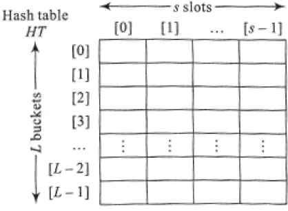
Figure 13.2 Hash table implemented using a sequential data structure
13.4.1. Operations on linear open addressed hash tables
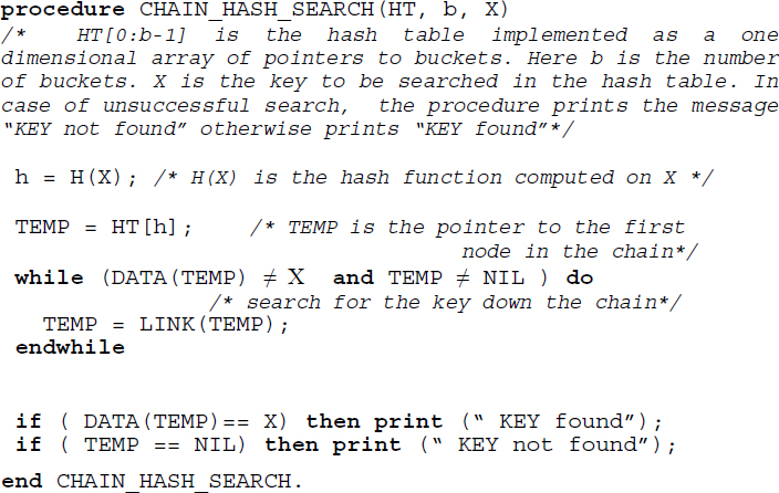
Search: Searching for a key in a linear open addressed hash table proceeds on lines similar to that of insertion. However, if the searched key is available in the home bucket then the search is done. The time complexity in such a case is O(1). However, if there had been overflows while inserting the key, then a sequential search has to be called which searches through each slot of the buckets following the home bucket until either (i) the key is found or (ii) an empty slot is encountered in which case the search terminates or (iii) the search path has curled back to the home bucket. In the case of (i), the search is said to be successful. In the cases of (ii) and (iii), it is said to be unsuccessful.
Algorithm 13.1 illustrates the search algorithm for a linear open addressed hash table.
Insert: the insertion of data elements in a linear open addressed hash table is executed as explained in the previous section. The hash function, which is quite often modulo arithmetic based, determines the bucket b and thereafter slot s in which the data element is to be inserted. In the case of overflow, we search for the closest empty slot beginning from the home bucket and accommodate the key in the slot. Algorithm 13.1 could be modified to execute the insert operation. The line
in the algorithm is replaced by
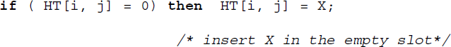
Delete: the delete operation on a hash table can be clumsy. When a key is deleted it cannot be merely wiped off from its bucket (slot). A deletion leaves the slot vacant and if an empty slot is chosen as a signal to terminate a search then many of the elements following the empty slot and displaced from their home buckets may go unnoticed. To tackle this it is essential that the keys following the empty slot be moved up. This can make the whole operation clumsy.
An alternative could be to write a special element in the slot every time a delete operation is done. This special element not only serves to camouflage the empty space ‘available’ in the deleted slot when a search is in progress but also serves to accommodate an insertion when an appropriate element assigned to the slot turns up.
However, it is generally recommended that deletions in a hash table be avoided as much as possible due to their clumsy implementation.
13.4.2. Performance analysis
The complexity of the linear open addressed hash table is dependent on the number of buckets. In the case of hash functions that follow modular arithmetic, the number of buckets is given by the divisor L.
The best case time complexity of searching for a key in a hash table is given by O(1) and the worst case time complexity is given by O(n), where n is the number of data elements stored in the hash table. A worst case occurs when all the n data elements map to the same bucket.
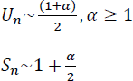
The time complexities when compared to those of their linear list counterparts are not in any way less. The best and worst case complexity of searching for an element in a linear list of n elements is respectively, O(1) and O(n). However, on average, the performance of the hash table is much more efficient than that of the linear lists. It has been shown that the average case performance of a linear open addressed hash table for an unsuccessful and successful search is given by
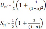
where Un and Sn are the number of buckets examined on an average during an unsuccessful and successful search respectively. The average is considered over all possible sequences of the n keys X1, X2, ….Xn.. α is the loading factor of the hash table and is given by ![]() where b is the number of buckets. The smaller the loading factor better is the average case performance of the hash table in comparison to that of linear lists.
where b is the number of buckets. The smaller the loading factor better is the average case performance of the hash table in comparison to that of linear lists.
13.4.3. Other collision resolution techniques with open addressing
The drawbacks of linear probing or linear open addressing could be overcome to an extent by employing one or more of the following strategies:
- Rehashing
A major drawback of linear probing is clustering or primary clustering wherein the hash table gives rise to long sequences of records with gaps in between the sequences. This leads to longer sequential searches especially when an empty slot needs to be found. The problem could be resolved to an extent by resorting to what is known as rehashing. In this, a second hash function is used to determine the slot where the key is to be accommodated. If the slot is not empty, then another function is called for, and so on.
Thus, rehashing makes use of at least two functions H, H’ where H(X), H’(X) map keys X to any one of the b buckets. To insert a key, H(X) is computed and the key X is accommodated in the bucket if it is empty. In the case of a collision, the second hash function H’(X) is computed and the search sequence for the empty slot proceeds by computing,
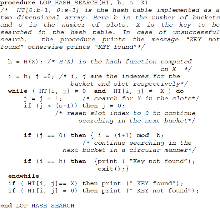
Algorithm 13.1 Procedure to search for a key X in a linear open addressed hash table
Here, h1, h2, ... is the search sequence before an empty slot is found to accommodate the key. It needs to be ensured that H’(X) does not evaluate to 0, since there is no way this would be of help. A good choice for H’(X) is given by M – (X mod M) where M is chosen to be a prime smaller than the hash table size (see illustrative problem 13.6)
- Quadratic probing
This is another method that can substantially reduce clustering. In this method when a collision occurs at address h, unlike linear probing which probes buckets in locations h+1, h+2 …. and so forth, the technique probes buckets at locations h+1, h+4, h+9,…. and so forth. In other words, the method probes buckets at locations (h + i2) mod b, i = 1, 2, …., where h is the home bucket and b is the number of buckets. However, there is no guarantee that the method gives a fair chance to probe all locations in the hash table. Though quadratic probing reduces primary clustering, it may result in probing the same set of alternate cells. Such a case known as secondary clustering occurs especially when the hash table size is not prime.
If b is a prime number then quadratic probing probes exactly half the number of locations in the hash table. In this case, the method is guaranteed to find an empty slot if the hash table is at least half empty (see illustrative problems 13.4 and 13.5).
- Random probing
Unlike quadratic probing where the increment during probing was definite, random probing makes use of a random number generator to obtain the increment and hence the next bucket to be probed. However, it is essential that the random number generator function generates the same sequence. Though this method reduces clustering, it can be a little slow when compared to others.
13.5. Chaining
In the case of linear open addressing, the solution of accommodating synonyms in the closest empty slot may contribute to a deterioration in performance. For example, the search for a synonym key may involve sequentially going through every slot occurring after its home bucket before it is either found or unfound. Also, the implementation of the hash table using a sequential data structure such as arrays limits its capacity (b × s slots). While increasing the number of slots to minimize overflows may lead to wastage of memory, containing the number of slots to the bare minimum may lead to severe overflows hampering the performance of the hash table.
An alternative to overcome this malady is to keep all synonyms that are mapped to the same bucket chained to it. In other words, every bucket is maintained as a singly linked list with synonyms represented as nodes. The buckets continue to be represented as a sequential data structure as before, to favor the hash function computation. Such a method of handling overflows is called chaining or open hashing or separate chaining. Figure 13.6 illustrates a chained hash table.

Figure 13.6 A chained hash table
In the figure, observe how the buckets have been represented sequentially and each of the buckets is linked to a chain of nodes which are synonyms mapping to the same bucket.
Chained hash tables only acknowledge collisions. There are no overflows per se since any number of collisions can be handled provided there is enough memory to handle them!
13.5.1. Operations on chained hash tables
Search: The search for a key X in a chained hash table proceeds by computing the hash function value H(X). The bucket corresponding to the value H(X) is accessed and a sequential search along the chain of nodes is undertaken. If the key is found then the search is termed successful otherwise unsuccessful. If the chain is too long maintaining the chain in order (ascending or descending) helps in rendering the search efficient.
Algorithm 13.2 illustrates the procedure to undertake a search in a chained hash table.
Insert: To insert a key X into a hash table, we compute the hash function H(X) to determine the bucket. If the key is the first node to be linked to the bucket then all that it calls for is a mere execution of a function to insert a node in an empty singly linked list. In the case of keys that are synonyms, the new key could be inserted either at the beginning or the end of the chain leaving the list unordered. However, it would be prudent and less expensive too, to maintain each of the chains in the ascending or descending order of the keys. This would also render the search for a specific key among its synonyms to be efficiently carried out.
Algorithm 13.2 Procedure to search for a key X in a chained hash table
Algorithm 13.2 could be modified to insert a key. It merely calls for the insertion of a node in a singly linked list that is unordered or ordered.
Delete: Unlike that of linear open addressed hash tables, the deletion of a key X in a chained hash table is elegantly done. All that it calls for is a search for X in the corresponding chain and deletion of the respective node.
13.5.2. Performance analysis
The complexity of the chained hash table is dependent on the length of the chain of nodes corresponding to the buckets. The best case complexity of a search is O(1). A worst case occurs when all the n elements map to the same bucket and the length of the chain corresponding to that bucket is n, with the searched key turning out to be the last in the chain. The worst-case complexity of the search in such a case is O(n).
On an average, the complexity of the search operation on a chained hash table is given by
where Un and Sn are the number of nodes examined on an average during an unsuccessful and successful search respectively. α is the loading factor of the hash table and is given by ![]() where b is the number of buckets.
where b is the number of buckets.
The average case performance of the chained hash table is superior to that of the linear open addressed hash table.
13.6. Applications
In this section, we discuss the application of hash tables in the fields of compiler design, relational database query processing and file organization.
13.6.1. Representation of a keyword table in a compiler
In section 10.4.1, (Volume 2) the application of binary search trees and AVL trees for the representation of symbol tables in a compiler was discussed. Hash tables find applications in the same problem as well.
A keyword table which is a static symbol table is best represented by means of a hash table. Each time a compiler checks out a string to be a keyword or a user-id, the string is searched against the keyword table. An appropriate hash function could be designed to minimize collisions among the keywords and yield the bucket where the keyword could be found. A successful search indicates that the string encountered is a keyword and an unsuccessful search indicates that it is a user-id. Considering the significant fact that but for retrievals, no insertions or deletions are permissible on a keyword table, hash tables turn out to be one of the best propositions for the representation of symbol tables.
13.6.2. Hash tables in the evaluation of a join operation on relational databases
Relational databases support a selective set of operations, for example, selection, projection, join (natural join, equi-join) and so on, which aid query processing. Of these, the natural join operation is most commonly used in relational database management systems. As indicated by the notation ![]() , the operation works on two relations (databases) to combine them into a single relation. Given two relations R and S, a natural join operation of the two databases is indicated as R
, the operation works on two relations (databases) to combine them into a single relation. Given two relations R and S, a natural join operation of the two databases is indicated as R ![]() S. The resulting relation is a combination of the two relations based on attributes common to the two relations.
S. The resulting relation is a combination of the two relations based on attributes common to the two relations.
One method of evaluating a join is to use the hash method. Let H(X) be the hash function where X is the attribute value of the relations. Here H(X) is the address of the bucket which contains the attribute value and a pointer to the appropriate tuple corresponding to the attribute value. The pointer to the tuple is known as Tuple Identifier (TID). TIDs in general, besides containing the physical address of the tuple of the relation also hold identifiers unique to the relation. The hash tables are referred to as hash indexes in relational database terminology.
A natural join of the two relations R and S over a common attribute ATTRIB, results in each bucket of the hash indexes recording the attribute values of ATTRIB along with the TIDs of the tuples in relations R and S whose R.ATTRIB = S.ATTRIB.
When a query associated with the natural join is to be answered all that it calls for is to access the hash indexes to retrieve the appropriate TIDs associated with the query. Retrieving the tuples using the TIDs satisfies the query.
Assume that a query “List the vendor(s) supplying the item P402” is to be processed. To process this request, we first compute H(“P402”) which as shown in Figure 13.11(b) yields the bucket address 16. Accessing bucket 16 we find the TID corresponding to the relation VENDOR is 7001. To answer the query all that needs to be done is to retrieve the tuple whose TID is 7001.
A general query such as “List the vendors supplying each of the items” may call for sequentially searching each of the hash indexes corresponding to each attribute value of ITEM_CODE.

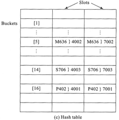
Figure 13.11 Evaluation of natural join operation using hash indexes
13.6.3. Hash tables in a direct file organization
File organization deals with methods and techniques to structure data in external or auxiliary storage devices such as tapes, disks, drums and so forth. A file is a collection of related data termed records. Each record is uniquely identified by what is known as a key, which is a datum or a portion of data in the record. The major concern in all these methods is regarding the access time when records pertaining to the keys (primary or secondary) are to be retrieved from the storage devices to be updated or inserted or deleted. Some of the commonly used file organization schemes are sequential file organization, serial file organization, indexed sequential access file organization and direct file organization. Chapter 14 elaborately details files and their methods of organization.
The direct file organization (see section 14.8) which is a kind of file organization method, employs hash tables for the efficient storage and retrieval of records from the storage devices. Given a file of records, { f1, f2, f3,……fN} with keys { k1, k2, k3,…kN} a hash function H(k) where k is the record key, determines the storage address of each of the records in the storage device. Thus, direct files undertake direct mapping of the keys to the storage locations of the records with the records of the file organized as a hash table.
13.7. Illustrative problems
Review questions
- Hash tables are ideal data structures for --------------------
- dictionaries
- graphs
- trees
- none of these
- State whether true or false:
In the case of a linear open addressed hash table with multiple slots in a bucket,
- overflows always mean collisions, and
- collisions always mean overflows
- true
- true
- true
- false
- false
- true
- false
- false
- In the context of building hash functions, find the odd term out in the following list:
Folding, modular arithmetic, truncation, random probing
- folding
- modular arithmetic
- truncation
- random probing
- In the case of a chained hash table of n elements with b buckets, assuming that a worst-case resulted in all the n elements getting mapped to the same bucket, then the worst-case time complexity of a search on the hash table would be given by
- O(1)
- O(n/b)
- O(n)
- O(b)
- Match the following:
- rehashing
- collision resolution
- folding
- hash function
- linear probing
- (A, i)) (B, ii)) (C, ii))
- (A, ii)) (B, ii)) (C, i))
- (A, ii)) (B, i)) (C, i))
- (A, i)) (B, ii)) (C, i))
- What are the advantages of using modulo arithmetic for building hash functions?
- How are collisions handled in linear probing?
- How are insertions and deletions handled in a chained hash table?
- Comment on the search operation for a key K in a list L represented as a
- sequential list,
- chained hash table, and
- linear probed hash table
- What is rehashing? How does it serve to overcome the drawbacks of linear probing?
- The following is a list of keys. Making use of a hash function h(k) = k mod 11, represent the keys in a linear open addressed hash table with buckets containing (i) three slots and (ii) four slots.

- For review problem 11, resolve collisions by means of i) rehashing that makes use of an appropriate rehashing function and ii) quadratic probing.
- For review problem 11, implement a chained hash table.
Programming assignments
- Implement a hash table using an array data structure. Design functions to handle overflows using i) linear probing, ii) quadratic probing and iii) rehashing. For a set of keys observe the performance when the methods listed above are executed.
- Implement a hash table for a given set of keys using the chaining method of handling overflows. Maintain the chains in the ascending order of the keys. Design a menu-driven front-end interface, to perform the insert, delete and search operations on the hash table.
- The following is a list of binary keys:

Design a hash function and an appropriate hash table to store and retrieve the keys efficiently. Compare the performance when the set is stored as a sequential list.
- Store a dictionary of a limited set of words as a hash table. Implement a spell check program that, given an input text file, will check for the spelling using the hash table-based dictionary and in the case of misspelled words will correct the same.
- Let TABLE_A and TABLE_B be two files implemented as a table. Design and implement a function JOIN (TABLE_A, TABLE_B) which will “natural join” the two files as discussed in section 13.6.2. Make use of an appropriate hash function.