
4
Optimization and Asymptotic Analysis of Insurance Models1
Insurance is the oldest domain of applied probability. Moreover, the mathematical models arising there can be used in other areas of applied probability. Therefore, the optimization of insurance models performance and their asymptotic analysis are very important. The modern period in actuarial sciences is characterized by the investigation of complex systems and the employment of sophisticated mathematical tools. Discrete-time models became popular since, in many cases, they describe more precisely the real situation. Hence, we study two models (the discrete-time one and the continuous-time one) in the framework of cost approach. Reinsurance, dividends and bank loans are the controls in optimization problems. Models stability with respect to small perturbations of underlying distributions is treated as well using the probability metrics.
4.1. Introduction
The investigation of insurance models is a primary task of actuarial sciences. A keyword in all definitions of actuarial sciences is risk. It is present whenever the outcome is uncertain, whether favorable or unfavorable. Actuarial sciences emerged in the 17th century (see Bernstein (1996)), although methods for transferring or distributing risk were practiced by Chinese and Babylonian traders as long ago as the 3rd and 2nd millennia BC, respectively. Actuarial sciences have an interesting history consisting of four periods (deterministic, stochastic, financial, modern – ERM (see Bulinskaya (2017)). As stated, the modern period is characterized by an investigation of complex systems and the employment of sophisticated mathematical tools. Discrete-time models became popular since, in many cases, they describe more precisely the real situation. They can also serve as the approximation of corresponding continuous-time models (see Dickson and Waters (2004)).
This chapter is organized as follows. In section 4.2, we consider a discrete-time insurance model with proportional reinsurance and bank loans. We establish the optimal policy of loans in the framework of cost approach and find the conditions for the model stability with respect to small perturbations of the underlying distributions. A continuous-time Cramér–Lundberg model with dividends is treated in section 4.3. An optimal barrier is found for the special type of claims distribution. Numerical results are also provided. Our conclusion and further investigation directions are discussed in section 4.4.
4.2. Discrete-time model with reinsurance and bank loans
4.2.1. Model description
Suppose that the claims arriving to an insurance company are described by a sequence of independent identically distributed (i.i.d.) non-negative random variables (r.v.’s) {Xi, i ≥ 1}. Here, Xi is the claim amount during the ith period (year, month or day). Let F(x) be its distribution function (d.f.) having density φ(x) and finite expectation. Put, as usual, ![]() . The company uses proportional reinsurance with quota α and bank loans. If a loan is taken at the beginning of the period (before the claim arrival), the rate is k, whereas the loan after the claim arrival is taken at the rate r with r > k. Our aim is to choose the loans in such a way that the additional payments entailed by loans are minimized. Denote by M the premium acquired by the direct insurer (after reinsurance) during each period. If x is the initial capital (surplus, reserve), then f1(x), the minimal expected additional cost during one period, is given by
. The company uses proportional reinsurance with quota α and bank loans. If a loan is taken at the beginning of the period (before the claim arrival), the rate is k, whereas the loan after the claim arrival is taken at the rate r with r > k. Our aim is to choose the loans in such a way that the additional payments entailed by loans are minimized. Denote by M the premium acquired by the direct insurer (after reinsurance) during each period. If x is the initial capital (surplus, reserve), then f1(x), the minimal expected additional cost during one period, is given by
Clearly, equation [4.1] can be rewritten in the form:
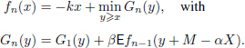
Now let fn(x) be the minimal expected cost during n periods and β be the discount factor for future costs. Then, using dynamic programming (see Bellman (1957)), we easily obtain the following relation:
4.2.2. Optimization problem
It is not difficult to prove the main optimization result.
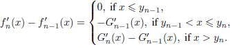
THEOREM 4.1.– There exists an increasing sequence of critical levels {yn}n ≥ 1 such that:
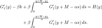
The sequence is bounded by y¯ satisfying the equation H(y) = 0 , where ![]()
PROOF.– Consider at first a one-period case. Obviously, we have to find the solution of the equation ![]() , where
, where ![]() . Due to assumption r > k, it follows immediately that y1 = αF−1 (1 – k/r) exists; moreover, it is the unique solution of the equation under consideration.
. Due to assumption r > k, it follows immediately that y1 = αF−1 (1 – k/r) exists; moreover, it is the unique solution of the equation under consideration.
Further results are obtained by induction. Since f1(x) is given by [4.4], it is possible to write
Hence, it is clear that ![]() for all x. Moreover, on the one hand,
for all x. Moreover, on the one hand,
on the other hand, we can write ![]() in the form:
in the form:
That means ![]() . Furthermore,
. Furthermore, ![]() for all x. Thus, the base of induction is established. Assuming that [4.4] is true for the number of periods less or equal to n, we prove its validity for n + 1. It is possible to write
for all x. Thus, the base of induction is established. Assuming that [4.4] is true for the number of periods less or equal to n, we prove its validity for n + 1. It is possible to write
Since
we deduce that ![]() , so yn < yn + 1. Rewriting
, so yn < yn + 1. Rewriting ![]() as follows:
as follows:

it is easy to see that ![]() . This entails the needed relation
. This entails the needed relation ![]() , thus ending the proof. It is possible to formulate an obvious corollary:
, thus ending the proof. It is possible to formulate an obvious corollary:
COROLLARY 4.1.– There exists ![]() .
.
REMARK 4.1.– It is interesting to mention that ![]() only for M = 0 whereas
only for M = 0 whereas ![]() for M > 0.
for M > 0.
4.2.3. Model stability
Now, we turn to sensitivity analysis and prove that the model under consideration is stable with respect to small perturbations of the underlying distribution. For this purpose, we introduce two variants of the model. In the first one, the claim distribution has density φX (x) and d.f. is denoted by FX (x). In the second one, the claim density is ϕY (x) and d.f. is FY (x). The corresponding cost functions are denoted by fn,X (x) and fn,Y (x). The distance between distributions will be measured by means of the Kantorovich metric.
DEFINITION 4.1.– For random variables X and Y defined on some probability space and possessing finite expectations, it is possible to define their distance on the base of the Kantorovich metric in the following way:
where FX and FY are the distribution functions of X and Y, respectively.
The distance between the cost functions is measured in terms of the Kolmogorov uniform metric. Thus, we are going to study.
To this end, we need the following:
LEMMA 4.1.– Let functions gi(y), i = 1, 2, be such that |g1(y) − g2(y)| < δ for some δ > 0 and any y, then supx| infy≥x g1(y) − infy≥x g2(y)| < δ.
PROOF.– Fix x and put Ci = infy≥x gi(y). Then, according to the definition of infimum, for any ε > 0, there exists y1(ε) ≥ x such that g1(y1(ε)) < C1 + ε. Therefore, g2(y1(ε)) < g1(y1(ε)) + δ < C1 + ε + δ implying C2 < g2(y1(ε)) < C1 + ε + δ. Letting ε → 0, we obtain immediately C2 < C1 + δ. In a similar way, we establish C1 < C2 + δ, thus obtaining the desired result |C1 − C2| < δ. Now, we are able to estimate Δ1.
LEMMA 4.2.– Assume κ(X, Y) = ρ, then Δ1 ≥ αrρ.
PROOF.– According to Lemma 4.1, we need to estimate |G1,X (y) − G1,Y (y)| for any y. The definition of these functions gives G1,X (y) − G1,Y(y) = r[E(αX − y)+ − ![]() . This leads immediately to the desired estimate. Next, we prove the main result demonstrating the model’s stability.
. This leads immediately to the desired estimate. Next, we prove the main result demonstrating the model’s stability.
THEOREM 4.2.– If κ(X, Y ) = ρ, then Δn ≥ Dnρ, where ![]() .
.
PROOF.– As in Lemma 4.2, we begin with the estimation of |Gn,X(y) − Gn,Y (y)| for any y. Due to definition [4.3], we have:

Obviously, the first term on the right-hand side of the inequality is less than αrρ. To estimate the second term, we rewrite it in the form:

Clearly,
Integrating by parts, we rewrite ![]() in the form:
in the form:

Hence, we obtain:
It is not difficult to prove that ![]() for all n, so:
for all n, so:
Solving this recurrent relation, we finish the proof and get the desired form of Dn.
COROLLARY 4.2.– ![]() for any n.
for any n.
In other words, we established the stability of the model with respect to small perturbations of claim distribution.
4.3. Continuous-time insurance model with dividends
4.3.1. Model description
In this section, we consider the classical Cramér–Lundberg model. Such a model was first introduced in 1903 by Lundberg (1903) and developed further in the 1930s of the last century by Cramér (1955). It was the beginning of the reliability approach (which is still popular) taking the ruin probability as a risk measure. It is a continuous-time model assuming that insurance company capital R(t) at time t is given by the relation:
where x = R(0) is the initial capital, Xn is the amount of the nth claim, and N(t) is the number of claims up to time t. The sequence {Xn, n ≥ 1} consists of i.i.d. non-negative r.v.’s with finite mean and d.f. F(x). It is independent of the Poisson process N(t) with intensity λ. The premium inflow rate is c > 0.
Starting with the seminal paper by De Finetti (1957), published in 1957, the study of dividends is an important subject for actuarial mathematics. We mention also in passing the papers by Gordon (1959) and Miller and Modigliani (1961), which were among the first to treat dividends problem, and the paper by Albrecher and Thonhauser (2009) which gives the review of results obtained before 2009.
Let us consider the Cramér–Lundberg process with dividends payed according to barrier strategy with level b. Then, the company capital at time t
where ![]() and L(t) is the dividend process satisfying the following conditions:
and L(t) is the dividend process satisfying the following conditions:
- 1) L(t + 0) − L(t) ≥ Q(t),
- 2) L(t)= L(T ) for all t ≥ T , where T = inf{t : Q(t) < 0} is the ruin time.
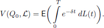
The objective function V(Q0, ℒ) is the expected discounted dividend payed until ruin. To calculate it, we introduce the following notation. Let ℒ be some strategy of dividend payment, Q0 be the initial capital, and δ be the force of interest, δ > 0. Then, it is possible to write:
DEFINITION 4.2.– The strategy ℒ0 is optimal if
4.3.2. Optimal barrier strategy
Further on we consider a barrier strategy.
DEFINITION 4.3.– The strategy ℒ is called barrier one with barrier level b, if for Q(t) > b, the amount Q(t) − b is payed immediately, if Q(t) = b, all the premium inflow is payed as a dividend and in case Q(t) < b nothing is payed.
We are going to use the following result proved in Gerber (1969).
THEOREM 4.3.– There exists b∗ such that for any initial capital satisfying condition 0 ≥ Q0 ≥ b∗ the barrier strategy specified by this level is optimal.
Put for simplicity Q0 = Q. Then, it is not difficult to prove using the total probability formula and properties of the Poisson process that V (Q, b) satisfies the following integro-differential equation:

with boundary condition:

We can find in the book by Bühlmann (1970) that the solution of [4.6] with boundary condition [4.7] has the form:
where function h(x) is a unique solution, up to a constant factor, of the equation

4.3.3. Special form of claim distribution
We have established that in order to find an optimal barrier strategy, it is necessary to solve two problems: to obtain the positive solution of [4.8] and calculate such a level b∗, that h′(b∗) is minimal.
THEOREM 4.4.– Assume that d.f. of claims has a density ϕ(y) given by ϕ(y) = P(y)e−y, y ≥ 0, where P(y) is the polynomial of degree m. Then, the integro-differential equation [4.8] can be reduced to a homogeneous ordinary differential equation of degree m +2 with constant coefficients.
PROOF.– Substituting in [4.8] expression dF(y) = φ(y) · dy, we have:
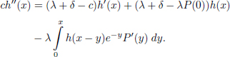
Differentiation gives the following relation:
Integration by parts of the last summand and replacement of the integral via formula [4.9] leads to:
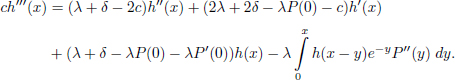
Note that we have already got a linear differential equation with constant coefficients plus the integral term. Performing the same transformation of expression [4.10], we obtain the differential equation of higher order:
Finally, to establish the relation between the function h(x) and its several derivatives, we repeat the previous cycle, getting:

Each time, we obtain the homogeneous linear differential equation with constant coefficients plus integral term. To make clear that such a statement is true for any order of equation, we write the following Table 4.1 showing how the new coefficients are related to those from the previous equation.
Table 4.1. Relations between coefficients
| ch′(x) | ch″(x) | ch‴(x) | ch(4)(x) | ... | |
| h(x) | λ + δ | λ − λP(0) + δ | λ − λP(0) − λP′ (0) + δ | λ − λP(0) − λP′(0) − λP″ (0) + δ | ... |
| h′(x) | 0 | λ + δ − c | 2λ + 2δ − λP(0) − c | 3λ + 3δ − 2λP(0) − λP′(0) − c | ... |
| h″(x) | 0 | 0 | λ + δ − 2c | 3λ + 3δ − λP(0) − 3c | ... |
| h‴ (x) | 0 | 0 | 0 | λ + δ − 3c | ... |
| ... | ... | ... | ... | ... | ... |
The lth column of Table 4.1 presents the coefficients in expression ch(l)(x) corresponding to h(x) (the first raw) and h(j−1)(x) (the jth raw), j ≥ 1. Hence, it is not difficult to see that the coefficients of the main diagonal have the form λ + δ − kc for non-negative integer k. It is clear from the procedure of getting the equation of order k + 1 from that of order k. The same reason is for the expressions in the first row of the table (coefficients by h(x), having the form λ + δ (in the first column) and λ(1 − P(0) − P′(0) −... −P(k)(0)) + δ (in the (k + 1)th column for any non-negative integer k)). In order to calculate the other non-zero coefficients (i.e. those on the main diagonal and above), we have to use the following rule: di,j = di,j − 1 + di−1,j−1 if di,j stands in the ith row and jth column. Obviously, all the coefficients are constant.
In all the equations along with derivatives, there exists an integral term. However, the order of derivative of polynomial P (y) under the sign of integral increases each time when we pass from the kth equation to the (k + 1)th one. Thus, using the induction, we obtain:
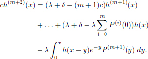
Since the (m + 1)th derivative of the polynomial is zero, the integral term disappears. It follows from the proved theorem that it is easier to find the optimal barrier for 0 ≥ Q ≥ b if the d.f. satisfies the condition dF(y) = e−y P(y) · dy, where P(y) is a polynomial of degree m. An example of such a distribution is Γ(m + 1, 1), where m is a non-negative integer. In this case, the density has the form ![]() .
.
An explicit solution is obtained for the case m = 0 (exponential distribution), whereas for m ≥ 1, numerical analysis is carried out. The program is written using Python programming language.
Therefore, we assume further that the claim amount has the exponential distribution with parameter γ, that is, F(y) = 1 − e−γy, where γ is the inverse of mathematical expectation. Since φ(y) = γe−γy (the polynomial degree is equal to zero), proceeding as in the general case, we obtain a homogeneous linear differential equation of the second degree with constant coefficients. In fact, we obtain
Let r1 and r2 be the roots of the characteristic equation:
The general solution of the differential equation under consideration has the form:
where C1 and C2 are constants to be determined.
Due to our assumptions, all the parameters are positive. It follows immediately that the signs of roots are different. For certainty, suppose that r1 > 0 and r2 < 0.
LEMMA 4.3.– The following relation holds:
PROOF.– We substitute the explicit form of h(x) in [4.8]. After calculation of h′(x) and integral in this equation, we set x = 0, obtaining:
According to Vieta’s theorem, we have ![]() , in other words,
, in other words, ![]() . Using this relation, we obtain 0 = (γ + r2)C1 + (γ + r1)C2. Whence it follows immediately that
. Using this relation, we obtain 0 = (γ + r2)C1 + (γ + r1)C2. Whence it follows immediately that ![]() has the desired form, thus ending the proof.
has the desired form, thus ending the proof.
The inequality r2 + γ > 0 is also valid. Therefore, according to Lemma 4.3 ![]() and constants C1 and C2 have different signs. Our aim is to find a positive solution h(x) for 0 < x < ∞. To this end, we need to have C1 > 0 (this is easy to understand, letting x tend to +∞ in the expression of h(x)), hence, C2 < 0 and C1 + C2 > 0 (we want to have h(0) > 0).
and constants C1 and C2 have different signs. Our aim is to find a positive solution h(x) for 0 < x < ∞. To this end, we need to have C1 > 0 (this is easy to understand, letting x tend to +∞ in the expression of h(x)), hence, C2 < 0 and C1 + C2 > 0 (we want to have h(0) > 0).
Thus, we established the form of h(x) and found the restrictions on the constants.
The last step is to find the optimal barrier b∗ in the set [0; +∞). In order to minimize the derivative h′(x), we have to find the root of the equation h∗″(x) = 0. Hence, we have to solve the following equation:
giving
The right-hand side is well defined, since we have already established that:
Thus, we have obtained the following expression:
4.3.4. Numerical analysis
We consider here the claim distributions with density φ(y) = γe−γy, that is, exponential distribution with parameter γ. To find the optimal barrier b∗, the formula [4.13] is used.
In the following, we provide the Python code for solving the problem of barrier calculation in a particular case and the results obtained:
import mathdelt = 0.05 # force of interestc = 1.1e6 # annual income (10 percent margin)lam = 1e3 # average NUMBER of claimsgam = 1e-3 # inverse average SIZE of a claimr = np.roots([c, -(lam+delt-c*gam), -delt*gam])barrier = math.log(((r[1]+gam)*r[1]*r[1])/((r[0]+gam)*r[0]*r[0]), math.e)/(r[0]-r[1])# roots of the equation print(barrier)>>> 112450.45449333431 # the optimal barrier
In Table 4.2, the optimal values of barrier b∗ are given for some parameters under the additional condition ![]() .
.
Table 4.2. Case 1
| 1/γ | λ | +5% | +10% | +15% | +20% |
| c = 1,050,000 | c = 1,100,000 | c = 1,150,000 | c = 1,200,000 | ||
| 100 | 10,000 | 25,705 | 16,392 | 12,571 | 10,454 |
| 500 | 2,000 | 93,674 | 64,050 | 50,440 | 42,574 |
| 1,000 | 1,000 | 156,529 | 112,450 | 90,094 | 76,750 |
| 5,000 | 200 | 424,339 | 375,834 | 322,837 | 284,878 |
| 10,000 | 100 | 573,129 | 588,160 | 532,745 | 482,573 |
The results for the case ![]() are given in Table 4.3.
are given in Table 4.3.
Table 4.3. Case 2
| 1/γ | λ | +5% | +10% | +15% | +20% |
| c = 5,250,000 | c = 5,500,000 | c = 5,750,000 | c = 6,000,000 | ||
| 100 | 50,000 | 32,530 | 19,944 | 15,043 | 12,387 |
| 500 | 10,000 | 128,526 | 81,962 | 62,857 | 52,269 |
| 1,000 | 5,000 | 227,297 | 148,555 | 115,041 | 96,199 |
| 5,000 | 1,000 | 782,644 | 562,252 | 450,470 | 383,749 |
| 10,000 | 500 | 1,253,205 | 965,726 | 792,042 | 682,949 |
In both cases, we calculated c in such a way that there will be a safety load of 5%, 10%, 15% and 20%. Note that the increase of safety loads leads to the decrease of the optimal barrier level.
4.4. Conclusion and further research directions
In section 4.2, we have investigated a discrete-time model and established its stability with respect to small perturbations of underlying distribution in terms of the Kantorovich metric. Moreover, we carried out the optimization of company performance in the framework of cost approach, proving that the best strategy of bank loans is determined by an increasing sequence of critical levels. However, we supposed that the quota share type reinsurance treaty is the same for all periods. The next steps are the consideration of non-proportional reinsurance and the search for optimal reinsurance depending on the length of the planning horizon. It is also interesting to deal with other metrics and prove the limit theorems, as in Bulinskaya and Gusak (2016).
A problem, proposed in the book by Bühlmann (1970), is solved in section 4.3. The company capital is described by a compound Poisson process controlled by dividend strategy. The expected discounted dividends until ruin are chosen as the objective function. For the barrier strategy, the explicit form of the linear differential equation is established if the claim amounts have the density φ(y) = P(y)e−y, where P(y) is a polynomial of degree m. Gamma-distributions with integer parameter belong to this class. Further investigation includes the sensitivity analysis of such a model and the consideration of more complicated models including dependence between the claim amounts and their number, investment in risky and non-risky assets and taxes. Other dividend strategies can be considered (see Bulinskaya (2018)). Due to a lack of space, these results will be published in another paper.
4.5. References
Albrecher, H. and Thonhauser, S. (2009). Optimality results for dividend problems in insurance. Revista de la Real Academia de Ciencias Exactas, Fisicas y Naturales. Serie A. Matematicas, 103(2), 295–320.
Bellman, R. (1957). Dynamic Programming. Princeton University Press, Princeton, NJ.
Bernstein, P.L. (1996). Against the Gods: The Remarkable Story of Risk. John Wiley and Sons, Inc., New York.
Bulinskaya, E. (2017). New research directions in modern actuarial sciences. Springer Proceedings in Mathematics and Statistics, 208, 349–408.
Bulinskaya, E. (2018). Asymptotic analysis and optimization of some insurance models. Applied Stochastic Models in Business and Industry, 34(6), 762–773.
Bulinskaya, E. and Gusak, J. (2016). Optimal control and sensitivity analysis for two risk models. Communications in Statistics – Simulation and Computation, 45, 1451–1466.
Bühlmann, H. (1970). Mathematical Methods in Risk Theory. Springer, Berlin, Heidelberg, New York.
Cramér, H. (1955). Collective Risk Theory: A Survey of the Theory from the Point of View of the Theory of Stochastic Process. Ab Nordiska Bokhandeln, Stockholm.
De Finetti, B. (1957). Su un’impostazione alternativa della teoria collettiva del rischio. Transactions of the XV International Congress of Actuaries, 433–443.
Dickson, D.C.M. and Waters, H. (2004). Some optimal dividends problems. ASTIN Bulletin, 34, 49–74.
Gerber, H. (1969). Entscheidungskriterien fur den zusammengesetzten Poisson-Prozess. Schweizerische Vereinigung der Versicherungsmathematiker Mitteilungen, 69, 185–228.
Gordon, M.J. (1959). Dividends, earnings and stock prices. Review of Economics and Statistics, 41, 99–105.
Lundberg, F. (1903). Approximerad Framstallning av sannolikhetsfunktionen. Aterforsakering av Kollektivrisker. Akad. Afhandling, Almqvist o. Wiksell, Uppsala.
Miller, M.H. and Modigliani, F. (1961). Dividend policy, growth, and the valuation of shares. The Journal of Business, 34(4), 411–433.
Chapter written by Ekaterina BULINSKAYA.
- 1 Research is partially supported by the Russian Foundation for Basic Research, project 20-01-00487.