5
Statistical Analysis of Traffic Volume in the 25 de Abril Bridge
Bridges are important structures. They are used on land transportation to connect different points that are usually inaccessible. Loading forces due to traffic volume and flow are important physical factors that affect the bridge’s structural reliability. Thus, for safety assessments, it is important to monitor and study traffic volume. In this work, we analyze the traffic data on the 25 de Abril Bridge in Portugal. The aim is to study the tail distribution.
5.1. Introduction
Bridges are the structures that allow people and vehicles to cross a space between two elevations. They are used to join roads, as well as to connect the two banks of a body of water, like a lake or river, or a deep opening, like a valley. The assessment of the safety of existing bridges has received technical and scientific attention, partly due to the occurrence of grave accidents in these structures. For safety assessments, it is thus important to monitor and study traffic volume and flow on bridges. In this work, we analyze the traffic volume data on the 25 de Abril Bridge, in Portugal (Figure 5.1). One main concern is the analysis of high traffic since it can lead to long periods of traffic congestion which can result in higher probabilities of failure of the bridge in its lifetime. The 25 de Abril Bridge opened on the 6th of August 1966 and connects Lisbon to the southern side of the Tagus River. This is the longest suspension bridge in Europe, with a total length of 2,277 meters. It has two levels: the upper level for cars with a three-lane roadway in each direction with a dividing guardrail as well as a lower one, built-in 1999, for trains. Due to its similarity and because it was manufactured by the same company, it is often compared to the Golden Gate Bridge in San Francisco.
The rest of this chapter is organized as follows: in section 5.2 we describe the data under study. In section 5.3, we review the extreme value methodology used in this work. Finally, in section 5.4, we apply the extreme value models to infer the extremal behavior of the traffic volume and provide some concluding remarks.

Figure 5.1. 25 de Abril Bridge and the Sanctuary of Christ the King monument (to the right of the photo) in the city of Almada. The photo was taken by the first author in September 2019. For a color version of this figure, see www.iste.co.uk/zafeiris/data1.zip
5.2. Data
The traffic data we considered in our analysis was provided by INE (Instituto Nacional de Estatística/Statistics Portugal) and by IMT (Instituto da Mobilidade e dos Transportes, I.P.). Although there are only tolls in the South-North direction, traffic is also counted in the other direction through sensors placed on the floor. The available data consists in the number of vehicles. No information is available regarding the class of a vehicle and the corresponding load. INE provided an archive of public data with easy online access. Regarding traffic volume, the data obtained from INE consists in the annual and monthly average daily traffic between 1998 and 2019. To study variations in the traffic, including the extreme values, the daily average could be meaningless. Thus, daily (or hourly) observations are more appropriate to make inferences in the right tail. Daily values since January 1, 2010 to December 31, 2018 were provided on request by IMT. We also obtained from IMT annual and monthly average daily data for the years before 1998.
Figure 5.2 shows the annual average daily traffic from 1966 to 2019. The years from 1966 to 2001 corresponds to a period of traffic growth. After 2001, the annual average daily traffic number appears to be stationary, with a change point in 2010. Note that the year 2001 corresponds to the beginning of the Portugal economic downturn and 2010 corresponds to the beginning of the sustainability financial crisis. In Figure 5.3, we present the time series plot of the daily traffic volume. The plot evidence shows strong seasonality within each year. The traffic volume is smaller in the winter months (December–February) and higher in the summer months (June–August). The three smallest values occurred on February 9, 2014 (82,408 vehicles), March 20, 2016 (82,654 vehicles) and March 11, 2018 (88,765 vehicles). The smallest number of vehicles was a consequence of the strong wind: the central lanes were closed, and traffic was closed to motorcycles and vehicles with canvas hoods. The other two dates coincide with the Lisbon Half Marathon where the bridge was closed to vehicles for several hours. The highest number of vehicles registered in the period 2010–2018 occurred on July 2, 2010 (180,846 vehicles).

Figure 5.2. Annual average daily traffic volume for the 25 de Abril Bridge, between 1966 and 2019
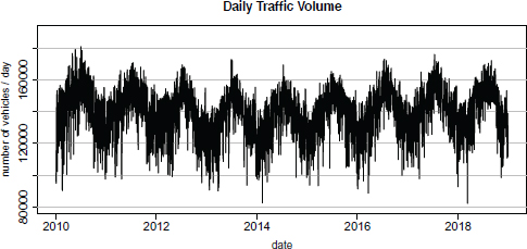
Figure 5.3. Daily traffic volume for the 25 de Abril Bridge, between January 1, 2010 and December 31, 2018
5.3. Methodology
The objective of extreme value theory (EVT) is to quantify the stochastic behaviour of extreme events, such as extreme climate events, a stock market crash or a new world record in athletics. The domains of application of EVT are quite diverse and include fields such as biology, hydrology, meteorology, geology, insurance, finance, structural engineering, sports and telecommunications. Thus, EVT provides a framework to model the tail behaviour and a tool to predict the likelihood of extreme events.
5.3.1. Main limit results
Let (X1,... , Xn) be a sample of independent and identically distributed (iid) random variables from an underlying population with unknown distribution function (df) F. Here, and due to the nature of the problem under study, we will always deal with the right tail of F. Since:
results for the left tail can be easily derived from the analogous results for the right tail. Fréchet (1927) and Fisher and Tippett (1928) were the first to derive asymptotic probability models for the transformed sample maximum. The first fundamental limit result is due to Gnedenko (1943) who fully characterized the three possible non-degenerate limit distributions of the linearly normalized sample maximum of iid random variables (see also von Mises (1964)1). This result is now known as the extremal types theorem. Let X(n) = max1≤i≤n(Xi) be the sample maximum. Let us also assume that there exist normalizing constants an > 0, bn ∈ ℝ and some non-degenerate df G such that, for all x,
With the appropriate choice of the normalizing constants, G must be one of the three limit models, which may be unified in the generalized extreme value (GEV) distribution,
here presented in the von Mises–Jenkinson form (Jenkinson 1955; von Mises 1964). When the non-degenerate limit in [5.1] exists, we say that F belongs to the max-domain of attraction of G and write ![]() . The shape parameter ξ is the extreme value index (EVI), the most important parameter associated with extreme events. This real parameter weights the upper tail of F . As ξ increases, the probability of occurrence of extreme values of X becomes higher. The GEV model unifies the three possible limit max-stables distributions: the Weibull (ξ < 0), the Gumbel (ξ = 0) and the Fréchet (ξ > 0). The GEV distribution is nowadays a common model for extreme value analysis since it covers all three forms of extreme value distributions.
. The shape parameter ξ is the extreme value index (EVI), the most important parameter associated with extreme events. This real parameter weights the upper tail of F . As ξ increases, the probability of occurrence of extreme values of X becomes higher. The GEV model unifies the three possible limit max-stables distributions: the Weibull (ξ < 0), the Gumbel (ξ = 0) and the Fréchet (ξ > 0). The GEV distribution is nowadays a common model for extreme value analysis since it covers all three forms of extreme value distributions.
Another important result in the field of EVT is the joint limiting distribution of the r largest order statistics (with r fixed). We will assume that equation [5.1] holds, i.e. (X(n) − bn)/an converges in distribution to G(x), with adequate normalizing constants an > 0 and bn ∈ R. Then, the joint limiting distribution of the normalized r largest order statistics is:
with X(n) ≥ X(n−1) ≥ … ≥ X(n−r+1), is the multivariate GEV model (Dwass 1964), with an associated probability density function given by:
if x(n) > x(n−1) > ... > x(n−r+1), where ![]() , and G(x) is the GEV distribution given in [5.2]. Note that for r = 1, equation [5.3] corresponds to the density function of the GEV distribution, as expected. Also, if we consider the extreme order statistic X(k) for some fixed k, we have (Arnold et al. 1992):
, and G(x) is the GEV distribution given in [5.2]. Note that for r = 1, equation [5.3] corresponds to the density function of the GEV distribution, as expected. Also, if we consider the extreme order statistic X(k) for some fixed k, we have (Arnold et al. 1992):
If k = 1, the limit distribution in equation [5.4] is the GEV distribution in equation [5.2]. There is thus a strong relationship between the asymptotic distribution of the sample maximum, X(n), the asymptotic distribution of the r largest order statistics and the extreme order statistic X(n−k+1), with k fixed. Other important limit results outside the scope of this paper can be found in other books (Leadbetter et al. 1983; Arnold et al. 1992; Coles 2001; David and Nagaraja 2003; de Haan and Ferreira 2006). For an overview of several topics in the field of EVT, see Beirlant et al. (2012), Davison and Huser (2015) and Gomes and Guillou (2015).
5.3.2. Block maxima method
The block maxima method consists of dividing the initial sample into disjoint blocks of equal size and fitting the GEV model in equation [5.2] to the sample of block maxima. The size of the block is important due to the usual trade-off between bias (small block size) and variance (large block size). When working with time-series data, it is usual to choose the block length as one year. This choice allows us to assume that the block maxima is iid, even though data has serial dependence. The limit in equation [5.1] justifies the following approximation, for large values of n:
Because the GEV model provides only an approximation for the distribution of Mn, bias due to model misspecification can occur. Since the normalizing constants an > 0 and bn ∈ ℝ are unknown, they are incorporated in the GEV distribution as location and scale parameters, λ and δ, leading to the model:
Next, we fit the GEV model in equation [5.5] to the block maxima sample. The estimation of the parameters (ξ, λ, δ) is usually performed using the maximum likelihood method or the probability weighted moment (PWM) method (Hosking et al. 1985). Since the support of the GEV model may depend on its parameters, the asymptotic normality of the maximum likelihood estimators may not hold. However, if ξ > −0.5, the maximum likelihood estimators are consistent and asymptotically normal (Smith 1985). Regarding PWM estimators, consistency and asymptotically normality can be guaranteed for ξ < 1 and ξ < 0.5, respectively. Note that in practical applications, we often have −0.5 < ξ < 0.5. Additional asymptotic results for the block maxima method were recently presented in Bücher and Segers (2017) and Dombry and Ferreira (2019).
Model checking can be done with a histogram, a probability plot, a quantile plot or with a return level plot with empirical estimates of the return level function (see Coles (2001) and Reiss and Thomas (2007) for further details).
5.3.3. Largest order statistics method
When analyzing extreme values with the block maxima method, we often miss several extreme observations. This problem has motivated researchers to use more extreme values from the sample. Smith (1986) and Weissman (1978) were the first to make inference with a model based on the r-largest order statistics from each block. Under this approach, the initial sample is divided into blocks and we select the r-largest order statistics from each block. Then, the model in equation [5.3] with additional location and scale parameters λ and δ > 0 is fitted to the data. The estimation is usually performed by maximum likelihood. As with the choice of the block length, the choice of the parameter r accommodates a trade-off between bias (large r) and variance (small r). In practice, it is advisable not to choose r too large (Smith 1986).
REMARK 5.1.– Note that both probabilistic models used in sections 5.3.2 and 5.3.3 share the same shape, location and scale parameters, (ξ, λ, δ). Therefore, it is usual to estimate those parameters, using the r-largest order statistics method, and then incorporate those estimates in the GEV model in equation [5.5] to estimate other important parameters.
5.3.4. Estimation of other tail parameters
Estimation of the model parameters is an important first step for further inference in the tail. The second and most important step is to yield precise inference about the tail behaviour of F . More precisely, estimate parameters such as an upper tail probability, an extreme quantile or the right-endpoint of F, whenever finite.
An upper tail probability is the probability that the block maximum exceeds some high value yp with probability p (p small). The tail probability can be estimated by ![]() , where G is the GEV df in equation [5.5].
, where G is the GEV df in equation [5.5].
Extreme quantiles exceeded with probability p of the block maximum can be obtained by inverting the GEV df in equation [5.5] and replacing the parameters by the corresponding estimates,
The quantile q1−p is also the level expected to be exceeded on average once every 1/p years. We usually say that q1−p is the return level associated with the return period 1/p. A plot of the return period (on a logarithmic scale) versus the return level is called a return level plot.
Let ω = sup{x : F(x) < 1} denote the right endpoint of the GEV model. If ξ < 0, the right endpoint is finite and can be estimated by:
5.4. Results and conclusion
The models presented in section 5.3 will now be applied to the traffic data of the 25 de Abril Bridge. We will consider only the period where daily values are available (2010–2018). Due to yearly seasonality, the block is defined as one year.
All computations were done in R software, with package ismev (Heffernan and Stephenson 2018). Table 5.1 shows the maximized log-likelihood (ll0), parameters estimates and standard errors in parentheses of the GEV (r = 1) and a multivariate GEV model with 2 ≤ r ≤ 5.
Table 5.1. Maximized log-likelihood (ll0), parameters estimates and standard errors in parentheses of the GEV (r = 1) and multivariate GEV model with 2 ≤ r ≤ 5
| r | ll0 | |||
| 1 | −87.599 | 170,156.651 (1,409.031) | 3,778.887 (1,026.358) | −0.132 (0.240) |
| 2 | −168.730 | 172,045.883 (1,404.189) | 4,348.683 (664.485) | −0.346 (0.164) |
| 3 | −244.945 | 172,548.763 (1,255.496) | 4,071.888 (526.778) | −0.314 (0.148) |
| 4 | −318.084 | 172,636.307 (1,109.469) | 3,858.426 (464.409) | −0.277 (0.123) |
| 5 | −388.923 | 172,390.040 (986.444) | 3,546.707 (357.260) | −0.250 (0.097) |
Comparing the results, we note that both estimates and standard errors change with different values of r. The standard errors decrease as r increases. Due to a possible increase of bias, it is advisable to not let r be too large. Coles (2001) suggests choosing r as large as possible, subject to diagnostics of the fit.
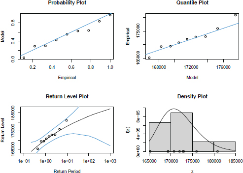
Figure 5.4. Diagnostic plots of the GEV model fit to the yearly maximum from the daily traffic data of the 25 de Abril Bridge. For a color version of this figure, see www.iste.co.uk/zafeiris/data1.zip
We validated the fitted model using the histogram, the probability plot, the quantile plot and the return level plot. These plots confirm that the fit is more satisfactory for r = 1. In Figure 5.4, we present the diagnostic plots of the GEV distribution based on the block maxima method (r = 1).
Using the delta method, the asymptotic 95% confidence intervals for the parameters ξ, λ and δ are, respectively, (−0.603, 0.338), (167395.0, 172918.3) and (1767.262, 5790.513). Despite the fact that the point estimate of the shape parameter ξ is negative, the corresponding confidence interval includes the value zero. Therefore, we do not have enough evidence to assume that the Weibull model is the most appropriate one. The likelihood ratio test statistic is equal to 0.292 which suggests that the Gumbel model could be adequate. Nevertheless, we decided to take the safest decision and prefer to model the tail within the GEV family of distributions.
In Table 5.2, we provide estimates and confidence intervals for the m-year return level (m = 10, 50, 100). Assuming the stationarity of future extreme values, we expect a daily traffic always below 195,000 vehicles during the next 100 years. Also, since the estimate of the shape parameter is negative, the endpoint estimate is 198,690 vehicles.
Table 5.2. Return period and estimates of the return level with 95% confidence interval
| Return period | Return level | 95% confidence interval for the return level |
| 10 | 177,511 | (173,115, 181,906) |
| 50 | 181,672 | (173,267, 190,076) |
| 100 | 183,175 | (172,367, 193,982) |
5.5. Acknowledgements
This work was partially funded by national funds through the FCT – Fundação para a Ciência e a Tecnologia, I.P., under the scope of the project UIDB/00297/2020 (Center for Mathematics and Applications).
5.6. References
Arnold, B.C., Balakrishnan, N., Nagaraja, H.N. (1992). A First Course in Order Statistics. Wiley, New York.
Beirlant, J., Caeiro, F., Gomes, M.I. (2012). An overview and open research topics in statistics of univariate extremes. Revstat – Statistical Journal, 10(1), 1–31.
Bücher, A. and Segers, J. (2017). On the maximum likelihood estimator for the generalized extreme-value distribution. Extremes, 20, 839–872.
Coles, S. (2001). An Introduction to Statistical Modeling of Extreme Values. Springer-Verlag, London.
David, H.A. and Nagaraja, H.N. (2003). Order Statistics, 3rd edition. Wiley, Hoboken, NJ.
Davison, A.C. and Huser, R. (2015). Statistics of extremes. Annual Review of Statistics and Its Application, 2(1), 203–235.
Dombry, C. and Ferreira, A. (2019). Maximum likelihood estimators based on the block maxima method. Bernoulli, 25(3), 1690–1723.
Dwass, M. (1964). Extremal processes. Annals of Mathematical Statistics, 35, 1718–1725.
Fisher, R.A. and Tippett, L.H.C. (1928). Limiting forms of the frequency of the largest or smallest member of a sample. Proceedings of the Cambridge Philosophical Society, 24, 180–190.
Fréchet, M. (1927). Sur le loi de probabilité de l’écart maximum. Annales de la Société polonaise de mathématique, 6, 93–116.
Gnedenko, B.V. (1943). Sur la distribution limite du terme maximum d’une série aléatoire. Annals of Mathematics, 44, 423–453.
Gomes, M.I. and Guillou, A. (2015). Extreme value theory and statistics of univariate extremes: A review. International Statistical Review, 83(2), 263–292.
de Haan, L. and Ferreira, A. (2006). Extreme Value Theory: An Introduction. Springer Science+Business Media LLC, New York.
Heffernan, J.E. and Stephenson, A.G. (2018). Package “ismev”: An introduction to statistical modeling of extreme values, version 1.42. Document, May 11.
Hosking, J., Wallis, J., Wood, E. (1985). Estimation of the generalized extreme value distribution by the method of probability-weighted moments. Technometrics, 27(3), 251–261.
Jenkinson, A.F. (1955). The frequency distribution of the annual maximum (or minimum) values of meteorological elements. Quarterly Journal of the Royal Meteorological Society, 81, 158–171.
Leadbetter, M.R., Lindgren, G., Rootzén, H. (1983). Extremes and Related Properties of Random Sequences and Processes. Springer-Verlag, New York, Berlin.
von Mises, R. (1964). La distribution de la plus grande de n valeurs. Selected Papers of Richard von Mises, American Mathematical Society, 2, 271–294.
Reiss, R.D. and Thomas, M. (2007). Statistical Analysis of Extreme Values: With Applications to Insurance, Finance, Hydrology and Other Fields, 3rd edition. Birkhäuser, Berlin.
Smith, R.L. (1985). Maximum likelihood estimation in a class of nonregular cases. Biometrika, 72(1), 67–90.
Smith, R.L. (1986). Extreme value theory based on the r largest annual events. Journal of Hydrology, 86, 27–43.
Weissman, I. (1978). Estimation of parameters and large quantiles based on the k largest observations. Journal of the American Statistical Association, 73, 812–815.
Chapter written by Frederico CAEIRO, Ayana MATEUS and Conceicao VEIGA DE ALMEIDA.
- 1 This reference is a reprint of the 1936 edition, found at: von Mises, R. (1936). La distribution de la plus grande de n valeurs, Rev., Math, Union Interbalcanique, 1, 141–160.