
4
Simulation Techniques Applied to the Analysis of Sociological Networks
4.1. Introduction
When exact methods cannot be used due to the complexity of the system, as observed or as conceptualized, recourse to simulation can make it possible to deal with more complex problems. This is the case with networks, the complexity of which may result from the interweaving of subnets. Simulation is often the only possible analytical approach, the complement of which is to produce results that cannot be generalized beyond the observations.
Computer simulation, now identified in the scientific community under the label M&S (Modeling and Simulation), is used to increase decision-making support capacities, especially for complex problems, that are difficult to handle by means other than computers. It is a question of approaching the behavior of a real or virtual dynamic system by means of a digital model, using the model as a platform for experiments, and then interpreting the results to make decisions on the system. A compilation of historical definitions on the concept of simulation is outlined in Pritsker (1979).
For a long time, driven mainly by practice, the field of M&S has remained in search of a general theory, to unify the diversity of approaches adopted, through the lens of a universal vision of the models, transversal to all fields of application, and with a coherent interpretation of all the transformations that characterize the evolution of a simulation model in its lifecycle. The very great heterogeneity, both of M&S methods and of the systems considered, acted as a brake to this unification. An important step was taken with the advent of paradigms, which laid down a solid foundation for the emergence of a real theory for M&S (Zeigler 1976).
4.2. Simulation techniques
The theorization of M&S is based on the unification of three paradigms (Figure 4.1):
- – A continuous-time specification of continuously evolving systems. This type of formalism is called a differential equation system specification (DESS).
- – A discrete-time specification of continuously evolving state systems. This type of formalism is called a discrete time system specification (DTSS).
- – A specification of discrete state evolution systems. With this type of formalism, only the times when the system changes state are retained (Discrete EVent system Specification, DEVS). However, the domain in which this time base takes its values can be continuous (a set of real numbers or a subset), or discrete (a set of integers or a subset), this second case (a finite state machine) can be viewed as a special case of the first.
It is possible to approximate a behavior specified in DESS by a DTSS specification, by discretizing time through intervals of fixed length. Continuous state changes are then approximated by stepped state changes. The evolution of the system between two bounds of an interval is approximated by a constant value (i.e. the state of the system at the start of this interval). The smaller the length of the intervals, the better the approximation, as well as the more expensive the computational burden. Conversely, the greater the length of the intervals, the less good the approximation, and the less expensive the computational burden. As such, the integration of a continuous function by the rectangle method is a DTSS discretization technique.
It is also possible to approximate a behavior specified in DESS by a DEVS specification, by discretizing the space of possible states by quantums of fixed length. This is why we speak of quantization. Each quantum represents a threshold that the state can reach and only those thresholds are observed (and not what becomes of the state between two thresholds). The times when these thresholds are reached then define the discrete values that time can take. To illustrate such an approximation, consider a vehicle’s fuel level as its state space. Instead of being interested in the evolution of this level in real-time (i.e. a DESS-type behavior), we are only interested in the moments when the vehicle tank is full, three quarters full, half-full, a quarter full, or empty. The times at which these thresholds are crossed depend on the type of driving and are therefore not necessarily at regular intervals (DEVS-type behavior).
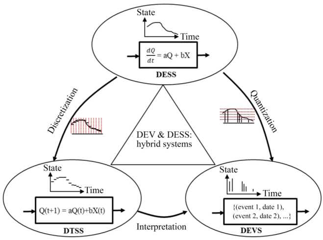
Figure 4.1. Modeling paradigms for simulation. For a color version of this figure, see www.iste.co.uk/bourrieres/networks.zip
It is of course possible, although generally more difficult, to switch from a DEVS or DTSS specification to a DESS specification. This is called interpolation (linear interpolations are quite easy to perform; other forms of interpolation are more difficult to express).
Moving from a DTSS to a DEVS specification, on the other hand, is only an interpretation of a DTSS as a special case of discrete time (DEVS).
Finally, in order to capture the full complexity of the evolution for the state of a system, it may be necessary to describe both the continuous and the discrete aspects. This is called a hybrid system, and a specification mixing both DEVS and DESS is said to be DEV&DESS.
COMMENT 4.1.– In this work, we are mainly interested in discrete event formalisms because they are naturally adapted to the specification of discrete flow networks.
4.2.1. Discrete event simulation (worldviews)
In a “discrete” simulation (DTSS and DEVS types), the model changes state at discrete points on the time axis. The simulation program implements all the state variables, whose values change over the simulation time according to rules defined in the model.
Historically, the expression worldviews has been used to characterize the three main approaches that have prevailed in building a simulation program, namely:
- – simulation by event scheduling;
- – simulation by process interaction;
- – simulation by activity scanning.
The first two techniques correspond to a DEVS specification and the last to a DTSS specification.
The prerequisites for event-driven simulation are:
- – identifying state variables – each state corresponds to a particular value for each state variable;
- – identifying the types of events – an event causes a change of state – and defining the logic for the state change that each event causes;
- – defining a simulation clock, the so-called virtual time, as opposed to the time of, say, a wall clock or that of the computer;
- – defining the rules to start and stop the simulation, and to calculate (often statistically) the results being observed.
The simulation program then consists of managing a schedule of planned events, sorted in ascending order the dates of when these events occurred, and a synchronization kernel. The synchronization kernel is a set of procedures to:
- – remove the event at the top of the schedule;
- – execute the corresponding state change and therefore update the state variables;
- – predict new events, to be included in the schedule in accordance with the sorting order;
- – cancel, if necessary, certain events and remove them from the schedule;
- – run the simulation, by time steps, from the date of an event occurrence to the date of the next event occurring in the schedule, and thus gradually calculate the results being observed.
Process-driven simulation is based on a synchronization kernel orchestrating the activation of processes for which only one can be active at a time. The execution of an active process performs the processing of schedule events under the remit of this process, and leads to the schedule update. The active process, at the end of treatment, is suspended and hands over to another process, which then becomes the active process. The suspended process is inserted in the list of paused processes, while the new active process is removed from this list. The simulation takes place by progressing in time jumps (from the occurrence date of a processed event to the occurrence date of the next event in the schedule), until reaching the stopping conditions.
In clock-driven simulation, the synchronization kernel is organized into activities that can be carried out at any time and simultaneously. These activities are associated with performance conditions. The clock is incremented in fixed time steps, and on each iteration, all conditions are scanned to determine the activities to be performed. The simulation thus progresses until it reaches the stopping conditions.
The advantage of the event-driven simulation approach is its simplicity, but has the disadvantage of requiring an exhaustive identification of event types. The process-driven simulation approach has the advantage of its intuitive nature, but the disadvantage of possibly complex interactions between processes. Finally, the clock-driven simulation approach has the advantage of modularity, but the disadvantage of slow execution.
In Tocher (1963), an attempt is made to reconcile the advantages of the different approaches presented above. Two types of activities are defined: “B-activities”, which correspond to primary events for which processing is unconditional and which can be programmed in advance, and “C-activities” which correspond to uncertain events whose processing is unconditional. The execution is subject to conditions, conditions checked at each stage of the simulation. On this basis, the simulation has three phases:
- – In Phase A, the next event in the schedule is removed and the clock is advanced to the corresponding occurrence date; all events with the same date of occurrence are also removed from the schedule.
- – In Phase B, all withdrawn events from the schedule and corresponding to B-activities are processed.
- – In Phase C, the conditions for triggering C-activities are tested and only those events which satisfy the conditions are processed.
4.2.2. DEVS formalism
A system is, according to the DEVS paradigm, a state machine. We consider a set of states S, finite or infinite, characteristic of the system, which interacts with its environment via a set of inputs X and a set of outputs Y. The state of the system evolves along a time base T⊂ R+.
At any time, the system is in the state s ∈ S with which we associate the total state (s, e) or e ∈ [0, ta(s)] indicating how long the system has been in the state s, this time not able to exceed a maximum value defined by a function ta called the time advancement function. The system leaves a state s, either at the end of the duration ta(s), or sooner, upon receipt of an input. The system thus changes state by external transition (in the case of an external stimulus) or by internal transition (at the end of the duration e ≤ ta(s)). These two types of transition are defined, respectively, by an external transition function δext and by an internal transition function δint which determine the successor state. Any reactions of the system to its environment are reflected in an output function λ which is only activated in the event of an internal transition.
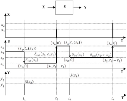
Figure 4.2. DEVS model dynamics
Figure 4.2 shows an example of the simultaneous evolution of the state, the inputs and outputs of the system, highlighting the laws that govern its behavior (functions of time advancement, transition and output): the graph of function X of T describes the trajectory of the inputs, the graph of function S of T describes the trajectory of states and the graph of function Y of T shows the trajectory of the outputs. At time t0 = 0, the system is in the initial state s3 and remains there until time t1 = 0 + ta(s3), since no input occurs before that date. The system then migrates by internal transition from the total state (s3,ta(s3)) to the total state (δint(s3),0), producing the output λ(s3). We have in this example δint(s3) = s1 and the system joins the total state (s3,0) on the date t1, for a maximum duration of ta(s1). As an input x1 occurs on a date t2 before the time limit ta(s1) has expired, the system migrates on this date by external transition from the total state (s1, t2 – t1) to a new total state, here (s4,0), determined by s4 = δext(s1,e,x1). And the life cycle of the system continues according to these same principles.
The operational semantics of DEVS models (atomic and coupled) – the formal specification given in section 2.9.1 – is defined by a protocol consisting of a hierarchy of Abstract Automata (called coordinators and simulators), under the control of a simulated time manager automaton (called the root coordinator) (Zeigler 1976). The simulators are in charge of generating the behavior for the atomic models and the coordinators the behavior for the coupled models. The simulation is carried out by sending messages (of different types and all stamped with their completion date) between the different automata, as described in Figure 4.3.
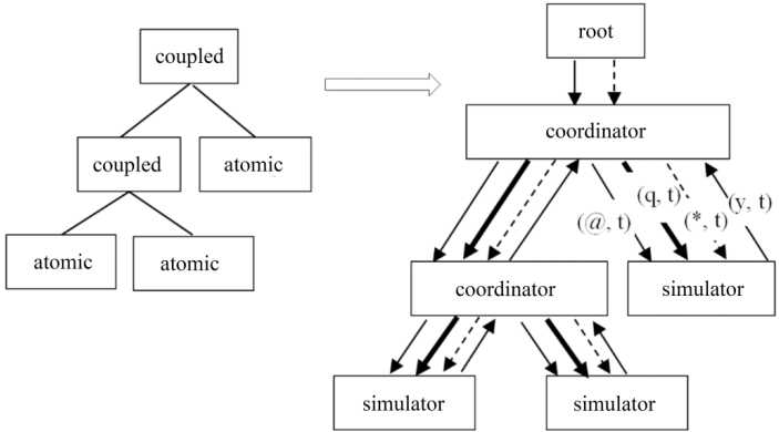
Figure 4.3. DEVS model hierarchy and simulation protocol
Table 4.1. Algorithm for the root
Initialize all components |
| t := tN from child |
| So long as the simulation is not over |
| Send (@, t) to child |
| Wait to receive (done, t) from child |
| Send (*, t) to child |
| Wait to receive (done, tN) from child |
The algorithms corresponding to the three types of automata (simulator, coordinator and root) are defined in an abstract way (Chow 1996), in order to leave the developer free to implement their strategy. Tables 4.1–4.3 give, respectively, the algorithms for the root, the simulators and the coordinators. Note that there are other versions of these algorithms, with different message types and calculation logics adapted to the strategies being adopted, without the overall principle of the protocol being called into question.
Table 4.2. Algorithm for a simulator (in charge of an atomic model)
| Message received | Actions to perform |
| (@, t) |
If t = tN then
Otherwise Error |
| (q,t) | Add the event q to the Bag for inputs Send (done, t) to the parent coordinator |
| (*, t) |
If tL ≤ t < tN and the Bag for inputs is not empty Then
Otherwise If t = tN and the Bag for inputs is empty Then
Otherwise If t = tN and the Bag for inputs is not empty Then
Otherwise If t > tN or t < tL Error Send (done, tN) to the parent coordinator |
Table 4.3. Algorithm for a coordinator (coupled model)
| Message received | Actions to perform |
| (@, t) |
If t = tN Then
Otherwise Error |
| (q,t) | Add the event q to the Bag for inputs |
| (*, t) |
If tL <= t < tN Then
Otherwise Error |
| (y, t) |
Using coupling
Wait to receive (done, t) from all these children Send (y, t) to the parent coordinator, if the coupling requires it |
4.2.3. Coupling simulation/resolutive methods
There are two kinds of complexity involved in the simulation analysis of a system:
- – Understanding and mastering the behavioral rules specific to the system, necessary for the modeling and then for the numerical simulation of the system, with a view to its evaluation, more precisely the instance of the model that results from the numerical values allocated to the model parameters. As indicated in section 2.9, one aspect of the specification of the simulation model is the mixture of modeling formalisms, some falling under a DESS-type approach, others of the DTSS or DEVS varieties. We then speak of hybrid simulation.
- – The difficulty linked to the very nature of the study, in terms of solving the question asked (difficult NP, complete NP, hard NP problems). It is necessary to have resolutive methods to guide the exploration of the parametric values of the model during iterative simulation campaigns of different instances of the model, until an instance that best meets the problem is found.
This double complexity, characteristic of the analysis of a system by coupling simulation/resolving methods (Figure 4.4), most often leads to the merger of concepts and methodological processes inspired by multiple disciplines (artificial intelligence, operational research, etc.) into a common approach, which immerses one or more simulation models into a decision-making device (human and/or a computerized analysis device). Coupling simulation/resolving methods responds to various engineering issues, for example (Traoré 2017):
- – performance evaluation (often seen as a discipline in its own right) which extracts quantitative knowledge on the behavior of a system;
- – intensive computing which, through the use of supercomputers, perform large simulation sequences (Monte Carlo simulations, resolution of large-scale digital models, such as those of fluid mechanics, civil engineering, climatic engineering, etc.);
- – virtual reality which is aimed at training and learning through animated visualization (opening up a wide avenue for advancement in medicine, robotics, aeronautics, military applications, emergency logistics, etc.).
The implementation of the coupling simulation/resolutive methods responds to the chronology shown in Figure 4.5, where we see two-time axes: the time shown by the wall clock as seen by the analyst, and the virtual time which is the temporality of the system being analyzed.
Centered simulation resolution process takes place along the “wall” time axis. We initialize the process by building a model, an instance of a class. In the most general case, the class is a parameterized model and the instance results from the choice of the numerical values for these parameters. For each model instantiation, a series of simulations (replications) is carried out.
As shown in Figure 4.4, each simulation requires initializing the model and defining the stopping conditions. The successive simulations each reproduce the dynamics of the model over a certain duration (Ti virtual time of the i-th simulation), which requires a certain experimental duration (τi execution time of the i-th simulation) in terms of the “wall” time. At the end of a series, a new instance is produced from new parameters and another sequence of experiments is carried out. Between each simulation, as well as between two model instantiations, different types of calculation can be performed: saving simulation results, carrying out specific processing for the calculation of performance indicators, etc.
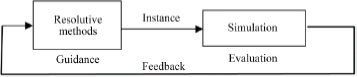
Figure 4.4. Coupling simulation/resolutive method diagram
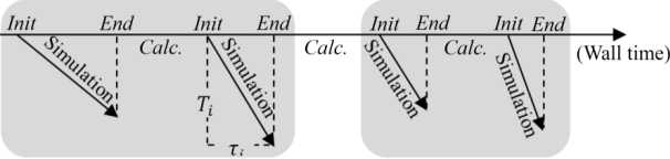
Figure 4.5. Implementation of coupling simulation /resolving methods
4.2.4. Distributed simulation
The heterogeneity of the modeling formalisms commented on in section 2.9 can be found at the simulation level. Distributed simulation aims to make the best use of the computational power of computers, to work on remote computers and to reuse existing simulations by interconnecting and orchestrating them. Indeed, as an interconnection of communicating components, networks naturally appear to be represented as components of a distributed simulation.
COMMENT 4.2.– We summarize here the main implications (architecture, distribution and synchronization of calculations, etc.) of distributed simulation, in response to network modeling and simulation needs. We refer the reader to Zacharewicz (2006) for additional information.
4.2.5. Architectural solutions
Among the architectural solutions suitable for distributed simulation, we can retain the use of a multiprocessor computer allocating part of its memory and computational capacity to each simulation component. It is also possible to interconnect several possibly remote computers (clustering). This architecture is isomorphic to the structure of networks and operates primarily by sending messages that allow simulation components to exchange data and to synchronize.
Different elements can be distributed in a simulation. We can indeed think of distributing certain functions of the simulator, or distributing events, or even distributing elements of the model. The latter solution makes it possible to reproduce the very infrastructure of networks, the simulator performing the execution of synchronized autonomous processes. In this case, we proceed by exchanging dated messages between the processes, which requires a message synchronization mechanism. We then make the best use of the parallelism inherent to the distributed architecture (Fujimoto 2000).
From the development of distributed simulation, environments and standards have emerged aimed at standardizing their construction. A first standard is distributed interactive simulation (DIS). The goal of DIS (Hofer and Loper 1995) is to relate heterogeneous simulations as entities that interact with each other through events.
The aggregate level simulation protocol (ALSP) (Miller 1995) is both a software and a protocol, aimed at allowing disparate simulations to communicate with each other. This protocol is used by the US military to link analytical and training simulations. Nevertheless, the reference standard for distributed simulation over the last two decades is undeniably high-level architecture (HLA) (see section 4.2.6).
4.2.6. Time management and synchronization
Distributed simulation is based on a set of logical processors (LP) which communicate by exchanging time stamped messages (events). Events can effectively represent material or information flows in a network. Each LP performs a local discrete event simulation, which maintains a timeline with local events and those received from other LPs, a current local state, and a local clock that contains the current local logical date.
Similar to sequential simulation, the evolution of time in distributed simulation can be synchronous or asynchronous. For synchronous evolution, the simulated time is given by a global clock which directs the local clocks of the LP, each associated with a node of the network. LP perform actions at each step of the global clock. In the case of an asynchronous evolution of time, the logical time of each LP evolves from event to event.
The parallel calculations implemented in distributed simulation make synchronization of the calculations necessary. Indeed, the simulated time is different on each LP; it is necessary to respect a principle of temporal causality (future events cannot influence with past events) to guarantee the consistency of the simulation. Lamport and Mahlki (2019) defines a causality rule applied to local logical clocks, requiring the arrival of an event a prior to an event b, implying that the local logical time C(a) is strictly less than the logical time C(b).
Respect for the principle of causality can be obtained using two types of the approach, presented below.
4.2.7. Pessimistic approach
An LP selects the local event (or the one received from an influencing LP) whose date T is the minimum date of its schedule. It processes this event by planning a new local event or to a destination intended for the influenced LPs, and updates the current logical date to the date of the processed event.
When an LP processes an event of date T, it must be sure not to receive other events of date T’ < T, and therefore respect the principle of causality. The goal of optimistic timing algorithms is therefore to determine which events are “safe” to process, the processing of which is not exposed to the occurrence of other events with a lower date (Bryant 1977; Chandy and Misra 1979).
The flaw of the pessimistic approach is that it does not exploit the full processing potential of the distributed simulation. Indeed, if an event a on a processor A is likely to affect an event b on a processor B, the synchronization algorithm must execute a and then b. If in fact a did not affect b, the simulator unnecessarily deprived itself of the simultaneous processing of a and b. “Safe” synchronization of processing therefore tends to sequence it, even when this is not necessary.
The simulation performance here is strongly linked to the setting of the lookahead duration during which an LP certifies that it will not send an exit message, thus giving up influencing the other LPs over this duration.
4.2.8. Optimistic approach
Contrasting with the previous approach, the optimistic approach allows the violation of the causal constraint. Each LP treats the events with a local and therefore partial knowledge of the events to be processed, which can lead to the omission of certain external events and the failure to respect causality (Samadi 1985). If a causal constraint is violated (receipt of an event whose date is prior to the current local date of the LP), the simulation then “returns to its past”, by means of a rollback mechanism (Jefferson and Sowizral 1985).
It can be noted that, at any time, the unprocessed message with the minimum date of all the LP deadlines is “safe”. Jefferson defines the date of this unprocessed message as the rollback point (Global Virtual Time, or GVT). All data relating to a date lower than the GVT is deleted, which frees up the memory occupied by backups, the final validation of actions, and thus the exploitation of the results of the simulation up until the GVT.
The shortcomings of the optimistic approach relate to the execution time spent making rollbacks that are often too large, and the need to store a large amount of data (events received, sent and states reached).
COMMENT 4.3.– There are approaches that combine optimistic and pessimistic approaches depending on the cost of using one method or another on the simulation.
4.2.9. HLA
Many complex simulations result from a combination of simulation components relating to different systems and include, additionally, interactions of these systems with the environment, for example, the simulation of human actors interacting within a physical environment in combat zones (Calvin and Weatherly 1996; Dahman 1997). Frequently, the simulations of some of these components already exist, developed for a particular purpose, and it may be interesting to reuse them in a new global simulation. Unfortunately, it is often necessary to make extensive modifications to adapt the model of a simulation component so that it can be integrated into a composite simulation. In some cases, it is even easier to perform a new simulation of the component than to modify the existing one. In other words, the desired properties of simulation components are their reusability and interoperability.
The reusability of simulation components allows them to be integrated into different simulation scenarios and applications, combining them with other components, without the need for recoding.
The interoperability of simulation components makes it possible for them to be executed by different types of interacting, distributed computational platforms.
This property involves rethinking the way simulation components interact, unlike a monolithic program running in a centralized computing environment.
The high-level architecture (HLA, IEEE Standard 2010), created by the American Department of Defense (DoD) for the requirements of military projects (Dahman et al. 1997), is a specification of software architecture making it possible to create simulations comprising different simulation components.
HLA realizes a federation of applications (i.e. federates) running on different platforms and interacting with each other. These federates are not only simulation applications, but also observer programs, acting as an interface with the real world to collect information, or interacting, for example, with a human operator.
In the HLA architecture, communication is established by sharing, broadcasting and receiving information. The typology of this information uses the concept of class resulting from object programming. The class of objects and their attributes designate the persistent data during simulation. The class of interactions and the associated parameters designate the non-persistent information exchanged between federates. A federate is an HLA-compatible computer program, the original code of which is supplemented by functions for communication with the other members of the federation. These functions are contained in the code of the FederateAmbassador class which allows federates to locally interpret information from the federation. A run time infrastructure (RTI) locally provides services to federates, such as object registration and time management, while the central component of the RTI manages the objects and interactions participating in the federation (Figure 4.6). The network structure chosen for execution consists of a central component and a set of peripheral federated components.
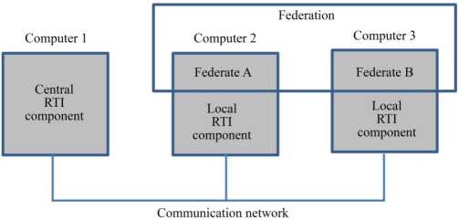
Figure 4.6. Two-federated high-level architecture. For a color version of this figure, see www.iste.co.uk/bourrieres/networks.zip
COMMENT 4.4.– Created in 1996, the HLA 1.3 standard evolved into the HLA 1516 standard in 2000, then to HLA 1516 Evolved (or HLA 1516-2010) in 2010. The HLA 1516-20XX (HLA 4) version is in preparation for 2022. Online courses for training in this standard are available (McLeod 1993).
4.2.10. Cosimulation
Often used in connection with distributed simulation, the term cosimulation primarily targets common interfaces that promote the interoperability of data exchanged between simulation components, without necessarily supporting the orchestration of these components. The synchronization of processors, which is one of the main topics in distributed simulation, therefore remains implicit in cosimulation and falls under the implementation of the solution.
In cosimulation, the different subsystems that form a coupled problem are modeled and simulated in a distributed manner. Cosimulation can be thought of as the joint simulation of already well-established tools and semantics when simulated with their appropriate solvers. Its advantage appears in the validation of multidomain and cyberphysical systems, by offering a flexible solution that allows us to consider several domains with different time steps, even though they are evolving simultaneously. In addition, by sharing the computational load between the simulators, it addresses the evaluation of large-scale systems. We present below the main standard of integration used in cosimulation.
4.2.11. FMI/FMU
Functional mock-up interface (FMI) is an open standard for the integration of heterogeneous simulation models in a standardized format. The FMI standard (FMI 2017) specifies an open format for the export and import of simulation models. This means that it is possible to select the most suitable tool for each type of analysis, while maintaining the same model. It is also possible to export a model to collaborators, who can reuse it for other applications and as tools specifically adapted to their needs, skills and preferences. Like HLA, this approach finds its origin in the valuation of portfolios, or libraries, of reusable simulation models for different applications.
Defined by the FMI standard, the FMU defines functional mock-up unit, in the form of computer files (“fmu” extension) which contain a simulation model conforming to the FMI standard. FMU files describe the behaviors of components and their interactions, in the form of binary code executable by different platforms or in the form of source code that can be compiled on different platforms targeted by the user.
The FMI standard specifies two different types of FMU:
- – Model exchange, (ME). The FMU ME represent dynamic systems by differential equations. To simulate the system, the import tool must connect the FMU to a digital solver.
- – Cosimulation (CS). The CS FMUs contain their own digital solver.
Figure 4.7 shows an FMI/FMU structure modeling a three-component network, including a master component and two running FMU components.

Figure 4.7. FMU structure and components. For a color version of this figure, see www.iste.co.uk/bourrieres/networks.zip
4.2.12. FMI/FMU and HLA coupling
The work of Gorecki et al. (2020) demonstrates the potential of a distributed simulation architecture associating HLA and FMI/FMU, applied to the complex case of a solar power plant. The proposed structure (Figure 4.8) includes a modeling and simulation orchestrator in association with a Papyrus modeling tool and a Moka execution engine dealing with the main process, in connection with a risk management federate that injects dysfunctional events into the distributed simulation.
The distributed and HLA simulations are connected to the JaamSim discrete event simulator, which reproduces the behavior of the solar power plant. Lastly, the platform is associated with a display tool that presents the results of the simulation.
Finally, the distributed simulation solution combines an HLA implementation framework to orchestrate Papyrus and JaamSim and, in addition, an FMI to orchestrate the Papyrus and FMU-Java App.
This example is indicative of the evolution of the state-of-the-art towards an ever-increasing interoperability to integrate simulation components into a logic of digital twins.
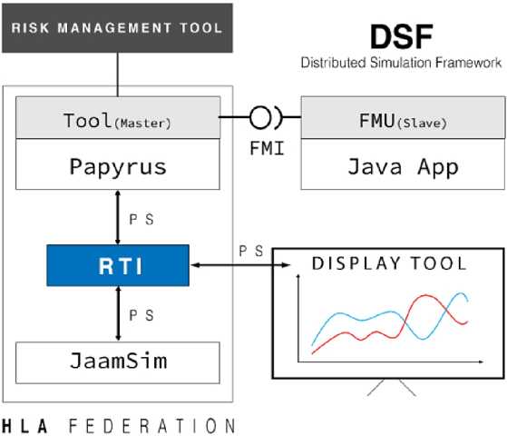
Figure 4.8. Example of HLA and FMI/FMU coupling (Gorecki et al. 2020). For a color version of this figure, see www.iste.co.uk/bourrieres/networks.zip
4.3. Simulation of flows in sociological networks
The multilayer sociological networks (MSNs) introduced previously (see section 2.7.3) are the basis of behavioral interactions via information propagation mechanisms, which can, to a certain extent, be simulated. In these models, the diffusion process is based on the interaction between network users subject to relationships of influence or social pressure.
Each node of the sociological network is associated with an individual, represented by an agent t. According to Ören (2020), the concept of agent computing is a natural paradigm for representing natural or artificial communicating entities with behavioral capabilities. Agent-based simulation is the use of agent technology to support modeling and simulation activities, as well as simulation-based problem solving.
Agents have a set of attributes:
- – Statistical attributes: gender, age, status, opinions, media (by which they can be attained), etc.
- – Dynamic attributes: interests, satisfied and unmet needs, according to the Maslow classification of human motivations (Maslow 1943).
COMMENT 4.5.– We describe here a general model of a sociological MSN network based on a set of agents and on the DEVS formalism (Bouanan et al. 2015a), as well as the implementation of a distributed simulator from an HLA architecture.
4.3.1. Behavioral simulation based on DEVS formalism
The propagation process develops from an initial situation where only a group of individuals have information that can be disseminated within the MSN to the rest of the population. Each message is a data packet with the following fields: source, destination, force and data. The concept of the force of a packet is a translation of the semantics of the message that may or may not mobilize the attention of the individual receiving it. If the message is of sufficient strength to be taken into account by the recipient individual, he or she can then relay it to other individuals in the MSN or not act upon it, depending on the interests of the recipients.
The packets thus circulate from one individual to another within the MSN, depending on the blocking behavior, or not, of the individuals.
A message is thus blocked in three possible situations:
- – The strength of the message is less than the detection threshold of the receiver.
- – The message is detected but not relayed due to the interests of other individuals.
- – The message arrives after a deadline and becomes out of date. The various thresholds must be set by the analyst.

Figure 4.9. DEVS model of reception/integration/distribution of an agent (Bouanan et al. 2015b)
The agent model and the DEVS formalism make it possible to specify the behaviors described above (Figure 4.9). A first state is used to configure and initialize the attributes of the agent, which then enters an “Idle” standby state. When the agent receives a message from another agent, it enters the “State 0” phase and the strength of the message is compared to a threshold value, which is an attribute of the agent. If the message strength is less than the threshold, the message is ignored by the agent and the agent returns to the “Idle” state. If, on the contrary, the threshold is crossed, the agent goes into “State 1” from which they can still – if they consider the message uninteresting for the other agents – give up relaying the message in which case it returns to the “Idle” state, or on the contrary, they decide to relay the message, which makes it pass into “State 2”, then into “State 3”, which triggers the transmission of a message to the other agents before returning to the “Idle” state.
4.3.2. Application study
The study presented here concerns the analysis of communication actions in a professional network and follows the work initially developed in the SICOMORES project (Constructive simulations and modeling of the effects of influence operations in social networks) (MASA 2013), led by the DGA (French General Delegation of the Armament) and which aimed to simulate communication operations and measure their influence in a context of conflict stabilization.
We consider here the relationships between people within a network of 10 companies of 30–50 people. Each company is broken down into four departments. These people are linked by three dimensions: collaborative ties within the same department, amicable ties within the same company and professional relations between different companies. Modeling the network leads to a three-layer MSN (Figure 4.10). The gray levels of the nodes represent the different companies to which people belong. The black, medium gray and light gray links represent, respectively, intra-department collaborations, amicable relations and professional relations between companies.
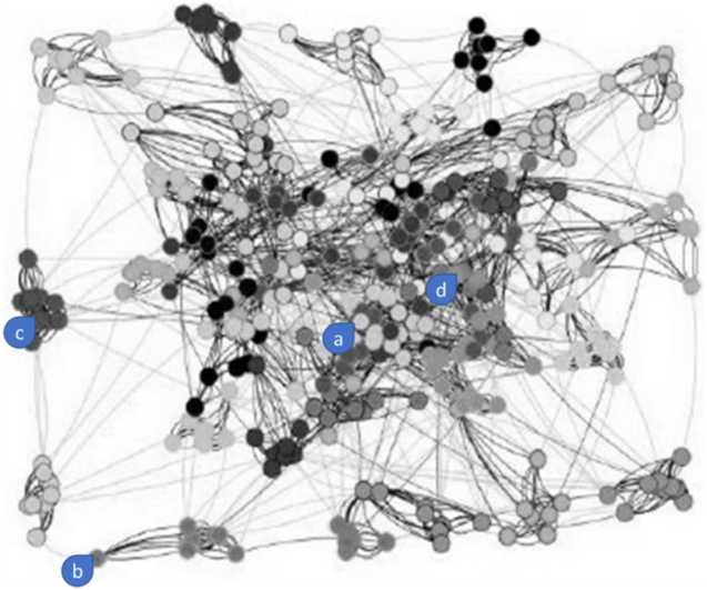
Figure 4.10. MSN from the professional network. For a color version of this figure, see www.iste.co.uk/bourrieres/networks.zip
The construction of the MSN is followed by the definition of the propagation rules for each layer of the network. Indeed, the propagation of messages differs according to the type of links between individuals.
The choice was made to maintain a separation between the different layers of the MSN, by representing each individual through a principal agent and through a proxy agent on each layer of the network. This solution is modular and transparent for each layer of the network in relation to the main agent model. In addition, each proxy agent can have its own rules for accepting and forwarding messages, so the primary agent may or may not be impacted by messages from different layers.
This principle made it possible to build an MSN simulator based on the VLE platform. We used the DEVS behavioral model presented above (Bouanan et al. 2015b) and is described in Figure 4.9.
The setting takes into account the description files of the network layers and their interconnection (MSN adjacency matrix), as well as an XML file containing the attributes of each individual. This file is used to initialize the population model by assigning to each agent the values of its attributes.
On the basis of these specification files, we built a distributed simulator of the MSN as an HLA federation with one federate per layer (Gorecki et al. 2020), set out in Figure 4.11.
The simulation of 600 simulated time units lasts less than eight hours on average, which is significantly less than a third of the duration for the undistributed simulation of the same problem performed elsewhere.
At the end of the simulation, a results file is generated, which contains the trace for the process of broadcasting all the messages (date of receipt of messages identifying receiving agents). The analysis of these data allowed us to analyze the scope, impact and dynamics of the dissemination of communication actions within the professional environment. The individuals with a strong influence according to their social and organizational position are certainly known a priori, but the simulation makes it possible to quantify their real influence. We were thus able to identify key individuals who do not have a particularly remarkable social or organizational status but who, located at the interfaces of several networks, are also very effective disseminators or relays of information.
We observe, for example (Figure 4.10), that a message sent by an individual-source “a” with a low level of responsibility manages to reach two-thirds of the population, and that a non-leader individual-source “b” only reaches 10% of the population. Conversely, a message sent by an individual “c” in a leadership position reaches two-thirds of the population, and the leader “d” manages to propagate a message to 80% of the population. This type of results was developed in Forestier et al. (2015).
We can thus measure the scope of information on the group from a transmitter. In real terms, within the professional field, this made it possible to study indirect distribution channels which are becoming increasingly important with the advent of social networks.

Figure 4.11. Distributed simulation of MSN (HLA architecture). For a color version of this figure, see www.iste.co.uk/bourrieres/networks.zip
4.4. Conclusion
This chapter presented simulation techniques, which remain the only recourse for the analysis of networks whose complexity does not allow for the use of exhaustive and complete resolution methods.
The simulation is only an evaluation tool, the vocation of which is to be used in an iterative manner, under the guidance of resolutive guiding methods that lead the analyst towards an almost optimal parameterization (in the subset of the scenarios simulated) of the system, taking into account certain objectives. This approach is the counterpart, in simulation, of the optimization approach using exact analytical methods.
By their multidimensional character and their particular logics for the propagation of information flows, social networks are an example of highly complex networks, which justify the use of distributed computing resources, capable of effectively simulating scenarios for the dissemination of messages in an MSN.
The DEVS behavioral models, the multidimensional social network and the resource sharing architecture for a distributed simulation presented in Bouanan et al. (2016) are open to the integration, if necessary, of more state variables in the agent models so as to more accurately describe human behavior in response to information received. Extensions of this model have thus been used in social science studies (Bergier et al. 2016a, 2016b; Ruiz-Martin et al. 2016), for healthcare networks (Sbayou et al. 2019), urban development networks (Bouanan et al. 2018) or to study the effectiveness of an emergency plan of a nuclear site (Ruiz-Martin et al. 2020).