
7
Introduction to Quantitative Data Processing and Analysis
This chapter presents the basic principles for the analysis of quantitative data. We start by describing how raw data is generally organized after the data collection. We then show that data follows a certain distribution, and we present one distribution in particular: the normal distribution. We also discuss the different ways to visualize and describe data. The second part of the chapter deals with data modeling for statistical tests, before describing the logic underlying such tests. Then, we briefly discuss some tests that have traditionally been applied to linguistic experimental data, and point out the inherent limitations in these. We see that nowadays there are more reliable models for analyzing this particular type of data, through the use of mixed linear models, for example. We present these models, as well as the results obtained with such analyses. We end the chapter by discussing some questions that may arise while analyzing data.
7.1. Preliminary observations
In Chapter 2, we saw that there are different types of variables which can be measured along different scales. The dependent variables used in linguistic experiments are generally measured along continuous scales, such as reaction or reading times, the number of items retained after reading a text, or an item’s acceptability on a scale from 1 to 10. Independent variables are often categorical in order to compare the data collected in the conditions of experiments. In this chapter, we will focus on the principles and analyses which are specifically related to this type of variable.
Data analysis requires a good understanding of different mathematical and statistical principles, the complexity of which can vary widely. In this introductory chapter, we will not be able to go into the detail of mathematical and statistical models. Hence, we encourage those interested in the concepts explained in this chapter to deepen their knowledge of them using the suggested reading at the end of the chapter.
Most of the analyses presented in this chapter also require the use of statistical software. Today, there is a very powerful and free access tool, R1 (R Development Core Team 2016), which has become the standard in language science. This software certainly requires a period of familiarization in order to understand and to learn how to apply the necessary codes for different functions. However, this training time quickly pays for itself, since the possibilities offered by R are prolific. Besides, R relies on a community of researchers who create and share packages, or in other words, reproducible code units, and who also provide documentation, software updating and technical support. When communicating the results of research, it is also increasingly expected to make available the data as well as the code on which the results are based, in order to favor the reproducibility and the openness of science. The use of R meets these expectations, enabling the proper management and recording of all the stages involved: processing, visualization and data analysis. Not only due to all the advantages mentioned, but also because this software is widely used within the scientific community, we encourage beginners to turn to R. An excellent basis to start learning statistics and to discover their application with R can be found in Winter’s book (2019), which is specially intended for researchers in language sciences.
7.2. Raw data organization
At the end of the data collection, a lot of data are integrated into one or more databases, depending on the technique used in the experiment. In order to illustrate a first possible type of database, let us consider the one devoted to participants, which should contain relevant demographic information identified by researchers. This database could take the form shown in Table 7.1 for participants 1 to 8 in a fictitious experiment.
Table 7.1. Example of a database describing the characteristics of participants

In this type of database, every row corresponds to one participant and every column is related to a demographic variable (age, mother tongue or laterality, for example) or to a variable included in the experiment (such as the list or condition assigned to each person, for example). In Table 7.1, we can see that lists were assigned to the participants in a sequential manner, as well as the conditions in which the experiment was carried out (in a solitary manner or in a group). In this example, we can also see a number representing each person. This is to respect the ethical principle of anonymity inherent in research. In fact, at no time should the identity of a participant be related to his/her performance in the task.
The data collected during the tasks themselves are presented in a similar way, except for the fact that every row now corresponds to an item in the experiment, rather than to a participant. In an experiment comprising 20 experimental items, 20 filler items and 20 participants, the database would thus include 800 rows, 40 for every participant and 20 for every item. This type of coding is called long format data. Table 7.2 illustrates, for one participant, the fictitious data obtained during a lexical decision task, in which word frequency and word length (in syllables) were manipulated. For every item included in the experiment, we can see the order in which it appeared, its type (experimental or filler item) and the different frequency and length conditions. The answers given by the participant and the time associated with every answer are also shown.
Table 7.2a. Example of a long format database (where one row corresponds to one item)
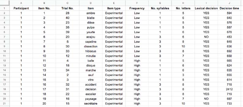
Table 7.2b. Example of a long format database (where one row corresponds to one item)

7.3. Raw data processing
Now that we have described different formats of raw databases, we will move on to the inspection of these data. Let us go back to the responses by participant #1 (Table 7.2) and take a look at them. We can see that the participant answered correctly in the majority of cases. In fact, there are only two NO replies related to words and three YES replies related to pseudo-words. The participant presents a correct response rate of 87.5% (35/40), suggesting that she has understood the task. This inspection of the responses given by the participants is an important step that should be carried out before analyzing the data, in order to exclude those who have not understood the task or who have not followed the instructions. The exclusion criteria should be clarified before observing the data, on the basis of theoretical principles, or the criteria used in prior research projects.
Now, let us take a look at this participant’s response times. These are generally around 700 milliseconds (ms), which further confirms that she followed the instructions and gave her answer quickly. Nevertheless, two response times are very far from the others. This is the case for item #17, associated with a response time of 2,412 ms, and item #24, with a time of 100 ms. Due to their distance from other response times, these particular measurements may not reflect the processes involved in a lexical decision task, but other processes. The time corresponding to 117 ms is very probably related to a participant’s error, who may have pressed the NO key prematurely. It seems highly unlikely that a person would be able to read the word and then categorize it in such a short time. The 2,412 ms time is more difficult to interpret. It could arise from a difficulty in processing, and then categorizing the word decision, thus suitably reflecting the processes investigated in the experiment. However, this time could also result from other processes, such as a decrease in concentration, for example. In the same way as the decision to exclude a participant from the experiment, the decision to exclude this type of response time must comply with the criteria chosen before data collection. We will return to this point later.
A final step before analyzing the data is to determine and to select which data will be analyzed. In this example on the lexical decision time, the data analysis should let us take a glimpse of the relationship between word recognition time and the variables word frequency and word length. In order to do this, only the word-related decision times should be taken into account, excluding the times related to non-words, as these were not related to the research question but were only used to make the lexical decision task possible. Among the response times for words, it is also necessary to consider only the times related to correct answers (or YES replies), showing that the words have actually been recognized as such.
7.4. The concept of distribution
The data acquired in an experiment can be summarized using different indicators. When communicating the results, it would be inappropriate to present all the individual data obtained in the experiment, as this would in no way be informative. Rather, a relevant summary of these data should be provided, thus enabling those interested to quickly understand the results. But before summarizing the data, it is essential to observe their distribution, that is, the frequency of the different values collected. This can be done through the use of a histogram, such as the one presented in Figure 7.1, which summarizes the fictitious data (YES correct responses) acquired for all the participants in the study described above, except for the extreme value.

Figure 7.1. Histogram representing the distribution of data acquired in an experiment. The black dashed line designates the mean of the distribution, whereas the gray dashed line is the median
On a histogram, different values are grouped into classes, the width of which can be adapted (here, the classes represent 20-ms intervals), and the height of which corresponds to the number of values contained in each class. Different types of information may be deduced from this histogram. First, the distribution has a single peak, between 750 and 770 ms, meaning that it is unimodal. Second, this peak is located at the center of the distribution and there is no positive or negative asymmetry. Third, we can observe that there are no extreme values located far from the other values. This distribution approximately corresponds to a normal distribution, since it is centered symmetrically around the central class, and presents a gradual decrease in the frequency of classes as we move away from the center. The normal distribution corresponds to a theoretical distribution for modeling the data observed empirically. It is generally represented by a probability density function, which indicates the probability of observing certain values. Two parameters, the mean and the standard deviation, define the distribution. The mean corresponds to the center of the distribution and indicates its location on the x axis. The standard deviation can be considered as the mean deviation around the mean. For a theoretical normal distribution, 68% of the data are located in the area between –1 and +1 standard deviation from the mean, 95% in the area between -2 and +2 standard deviations and 99.7 % in the area between –3 and +3 standard deviations (see Figure 7.2). This means that if a value were to be chosen randomly from such distribution, in 68% of the cases, it would correspond to a value placed within one standard deviation of the mean, and in 95% of the cases, it would correspond to a value placed within two standard deviations of the mean.

Figure 7.2. Normal distribution, with a mean of 0 and a standard deviation of 1
Many statistical tests are based on the normal distribution, as it corresponds to the form that likelihood takes. By analogy, we can estimate that many variables are distributed in a normal way in the population.
7.5. Descriptive statistics
To summarize the data, we generally report the center of the distribution, also known as the central tendency. The central tendency can be measured in three ways. A first way – which we have already discussed – is the mean, which can be simply obtained by adding the values and then dividing the total obtained by the number of values. For a normal distribution, the mean indicates the location of the center of the distribution. In our example, it would correspond to 765 ms (the black dashed line in Figure 7.1). However, the mean alone cannot summarize data in an informative manner because a distribution is also defined by its dispersion, which can be evaluated by the standard deviation, for example.

Figure 7.3. Graphic illustrations of decision times by participant #1 and the mean for correctly recognized experimental items (gray line). Panel (a) does not contain the extreme value of 2,412 ms, whereas panel (b) contains it
To illustrate this, let us consider the correct YES decision times by participant #1 and plot them on a graph. Figure 7.3, panel (a), shows the mean (gray line) for all the data concerning participant #1, with the exception of the time of 2,412 ms. We can see that every value deviates from the mean by a certain distance (arrow). In order to quantify the total distance, we might imagine adding the individual distances. However, this is not a good solution, since the distances of the values below the mean are compensated by those located above the mean, and their sum would therefore be equal to 0. In order to remedy this problem, it is necessary to transform negative values into positive ones, which can be achieved by squaring them. The variance of the sample is thus calculated on the basis of the sum of the squares of the distances from the mean, divided by the number of observations minus one. By calculating the square root of the variance, we obtain the sample’s standard deviation, which can be considered as an indicator of the average distance from the mean, which can be seen as the average error around the mean. In the example we are interested in, the mean is 649 and the standard deviation is 49. In other words, the central value of the distribution is 649 ms and the data move away from it by 49 ms on average. Let us now observe the effect on the mean and the standard deviation when we add the 2,412 ms value (Figure 7.3, panel (b)). Introducing this value into the calculation would increase the mean to 747 and the standard deviation to 418. This illustrates that a single value can strongly influence the mean and the standard deviation of a distribution. This type of value is called an extreme value.
Managing extreme values is a complicated issue for researchers. While there is general consensus that extreme values corresponding to impossible values, for example, resulting from a coding error, should be eliminated from the data, there is no clear procedure concerning extreme values such as the one we have here. In the literature, we find two ways for dealing with them, which can be combined in some cases. A first solution would be to exclude data outside an acceptable range that should be defined by researchers before the data collection, on the basis of theoretical criteria. For example, for a lexical decision task, several articles have reported the exclusion of times shorter than 200 ms and longer than 2,000 ms (e.g. Ferrand et al. (2010)). In this case, the criteria depend on the task or the type of process investigated and should be set for every new study.
A second solution, which can be implemented following the first, would be to eliminate or to replace extreme values on the basis of the distribution of the results. We can often read in the literature that for every participant and/or every item, data further than 2, 2.5 or 3 standard deviations from the mean have been eliminated or replaced by their threshold value. In the example we are discussing, the value of 2,412 deviates by more than 3 standard deviations from the mean. We could decide to eliminate this value or replace it with a less extreme value, like 2,002, which corresponds to the mean plus 3 standard deviations. Although we will not go into further detail in this book, it is important to note that the scientific community is not unanimous regarding the validity of this approach. For further developments, we refer those interested to McClelland (2014) who discusses these options, and to Leys et al. (2013) who present an alternative solution. In all cases, whatever the criteria chosen for the treatment of extreme values, these must be reported together with the results. In addition, it is customary to indicate the percentage of data that have been replaced or deleted.
The examples described above show that the mean is a good central tendency indicator when the data are distributed symmetrically. In other cases, it may be appropriate to summarize the data using another measure, such as the median. This simply corresponds to the value that separates the distribution into two equal parts. Half of the values are below the median, and the other half are above (the gray dashed line in Figure 7.1). Unlike the mean, the median is only slightly influenced by extreme values. If, for example, a third of the values in the distribution had values higher than 2,000 ms, the median would always remain the same. For this reason, this measure of central tendency is sometimes preferred to the mean when the distribution contains extreme data or when it follows an asymmetrical curve.
So far, we have considered all the correct YES decision times gathered in the experiment, regardless of the condition in which they were obtained. The fictitious study that we are examining, however, focuses on the influence of two variables, word length and word frequency, on decision times. It would therefore be more appropriate to observe the distribution of times in the different conditions resulting from the combination of these variables, as illustrated in Figure 7.4.

Figure 7.4. Histograms representing the decision times obtained in the different conditions of the experiment, as well as the mean for each condition (dashed line)
On these representations, we can see approximately normal distributions in the different conditions. We can also observe that, in general, the decision times for low frequency words (793 ms, bottom-line) are higher than those related to high frequency words (738 ms, top-line). The difference between short words (762 ms, right column) and long words (769 ms, left column) is very narrow. These results suggest that in our sample, it is only word frequency – not word length – that influences the lexical decision time.
7.6. Linear models
In order to represent data and to analyze the influence of independent variables on dependent variables, it is necessary to rely on models. A model makes it possible to predict the values of the dependent variable based on the values of the independent variable (also called predictor). In other words, a model aims to mathematically represent the relationship between two or more variables.
In this chapter, we will present statistics that are based on linear models. This simply means that the predicted data are summarized by a straight line. In order to define this line, it is necessary to determine its intercept, that is, the point where it crosses the y axis, as well as its slope, or the evolution that the line follows as the value of the predictor increases. For a model with only one predictor, the equation corresponds to:
In this equation, y represents the predicted value and x the value of the predictor; b0 is the intercept and b1 the slope of the straight line. The intercept corresponds to the value of y when x = 0, and the slope corresponds to the change in the value of y when the value of x changes by one.
A very simple model that we have already mentioned is the mean. In this model, only the intercept (the mean) is defined. If we predicted the decision times only on the basis of the mean, this prediction would be imprecise, because as we have already seen, the observed values never correspond exactly to the mean and deviate a certain distance. This difference between predicted and observed values is called error and is symbolized by ε in the equation.
In order to build a model that describes the data more accurately than the mean, we can add a regression coefficient b1 associated with a relevant predictor. Adding this predictor aims at reducing the model’s error. Figure 7.5 illustrates the participants’ mean decision time in low and high frequency conditions (where every point represents a participant). On panel (a), the line represents a model based on the mean. We can quickly notice that this model does not help in the prediction of observed times; it reflects data in general, without taking into account the specifics related to the conditions. On panel (b), a linear model was calculated, in order to include the role of frequency on decision time. This model is as follows:
In a model including categorical predictors, it is necessary to assign a value to their different modalities. The choice made on panel (b) corresponds to what is called dummy coding, in which a value of 0 is assigned to the reference modality and a value of 1 is assigned to the second modality (the order of the modalities is determined alphabetically in R). For the reference modality (high frequency), the equation simply predicts the mean time of this condition (738+54*0). Thus, we can see that the intercept is equivalent to the mean of the reference category. If we apply the equation to the second modality of the variable (738+54*1), we then obtain the mean of the low frequency condition. When dummy coding is used, the regression coefficient represents the difference between the means in the two conditions.

Figure 7.5. Mean decision times of participants in high and low frequency conditions. On graph (a), the line represents a model based only on the mean. On graphs (b) and (c), the model takes into account the frequency predictor, using two different codings for the predictor ((b) = binary coding, (c) = sum coding) The intercept corresponds to the white circle
Another possibility for coding categorical predictors is to use sum coding, which assigns opposite values to the modalities of the predictor, so that their sum is equivalent to 0.
In this type of coding, the value 1 corresponds to the reference category. In this specific case, value 1 is assigned to the high frequency condition and value -1 to the low frequency condition. This means that the intercept calculated in such a model no longer corresponds to the mean of the reference condition, but to the general mean, taking the times of the two conditions into account, as in equation [7.3], which corresponds to panel (c) in Figure 7.5.
When sum coding is used, the regression coefficient indicates the difference between the general mean and the mean in each condition. In this precise case, it would be necessary to subtract 27 ms (-27*1) to the intercept to obtain the mean of the high frequency condition, and to add 27 ms (-27*(-1)) in order to obtain the mean of the low frequency condition.
Linear models can also be built on the basis of several predictors. To do this, we can simply add a regression coefficient associated with one or more additional predictors to the equation, as in the following example:
If we included word length in the model, using sum coding, we would obtain:
When several predictors are included, it is possible to specify the terms of interactions between predictors. However, as we mentioned in the previous chapter, it is not recommended to include too many predictors in a model, especially when they involve interactions, because these models quickly become difficult to interpret.
The influence of the predictors included in the model is then tested using inferential statistics, whose logic we will describe in section 7.7.
7.7. Basic principles of inferential statistics
The primary goal of an experiment is to answer general questions and to reach conclusions that can be applied to a group of people or to a set of linguistic items. In the fictitious experiment we are discussing, the aim is to analyze the influence of word frequency and word length on the lexical decision time for people and words in general. However, in reality, it is impossible to test all the people or all the words. For this reason, data are collected from a sample of people, based on a sample of items. The parameters estimated at the sample level (means and standard deviations, for example) are then used to make deductions at the population level. There are different approaches for inferring conclusions for a whole population on the basis of a sample (Dienes 2008). The most common and widely used so far corresponds to the null hypothesis significance testing (NHST) framework.
7.7.1. The null hypothesis significance testing
In the NHST framework, the research hypothesis related to every independent variable of the study is expressed in the form of two opposite statistical hypotheses. The first one, the null hypothesis (H0), states that the independent variable does not influence the dependent variable. In other words, the means observed in the different conditions should be the same. The second one, the alternative hypothesis (H1), says that the independent variable influences the dependent variable. In other words, the means observed in the different conditions should differ. In order to illustrate these different hypotheses, let us go back to our example by imagining that we have examined the influence of a single variable, word frequency.
The statistical hypotheses in this situation would be as follows:
H0: the mean decision time for frequent words is equal to the mean decision time for less frequent words.
H1: the mean decision time for frequent words is different from the mean decision time for less frequent words.
It is important to note that these statistical hypotheses are not related to the sample from where the observed data were retrieved, but to the population for which one wants to draw conclusions.
The various statistical tests carried out within the NHST framework aim to check the compatibility of the data observed in an experiment with the data that would be predicted for the population by the null hypothesis. In our example, this logic would amount to saying “if word frequency did not influence decision time, what would be the probability of observing a difference of 54 ms between the conditions in our sample?”. In order to answer this question, the statistical tests are based on the models we mentioned in the previous section. They are generally carried out on the basis of the difference in means between conditions, as well as on the basis of variations in data and sample size. Actually, a difference between means, as in our example, may be related to two possible sources. The first source corresponds to the systematic variation in the data that can be attributed to the manipulation, or in other words, to the fact that the word was frequent or not. The second source of variation corresponds to the unsystematic variation in the data, which can be attributed to the participants, such as their being faster/slower to respond, or to the items, such as being more or less familiar, for example.
In a simplified way, statistical tests in the NHST framework calculate the ratio between the systematic variation and the unsystematic variation explained by the model. If this ratio is greater than 1, this means that the systematic variation is greater than the unsystematic variation and that the independent variable has an effect. In order to know whether this effect is significant, the value returned by the statistical test is compared with a sampling distribution specifically related to the test performed. This makes it possible to determine the probability of observing an equal result or a more extreme result than the one observed in our sample if H0 were true, which is called the p-value. If the p-value is small enough, then it is possible to reject the null hypothesis. In a relatively arbitrary manner, the majority of the scientific community has set a threshold below which the p-value would be acceptable, conventionally placed at 0.05 in Human Sciences. When p is smaller than 0.05, a result is said to be statistically significant.
The p-value is a conditional probability since it represents the probability of obtaining the observed data (or more extreme data) if H0 were true. It is very important to remember this, so as not to draw the wrong conclusions from the p-value. In sum, the p-value gives no indication of the probability of H0 being true. The null hypothesis is only a theoretical distribution and it is not possible to take a stand as to its veracity. Likewise, the p-value does not let us express an opinion as to the veracity of H1. Indeed, the p-value only provides an indication as to the compatibility of the data observed with H0, nothing else. Finally, the p-value does not directly reflect the size of an effect. For this reason, and in order to better interpret the statistical effects discovered, it is essential to couple the p-value with other measurements we will describe below.
7.7.2. Effect sizes and confidence intervals (CIs)
Imagine that, in our example, the difference observed between the frequency conditions is statistically significant, that is, that the p-value associated with the 54 ms difference is smaller than 0.05. The importance of this difference can be estimated on the basis of several points, as described by Winter (2019). First, it can correspond to the magnitude of the difference itself, here 54 ms. The greater this magnitude, the more the effect can be considered as important. Second, the importance of the difference depends on the variability observed in data: when the variability is small (reflected by a small standard deviation), we can be more confident about the existence of the difference than when the variability is large. These two points can be combined in order to calculate effect size statistics, which helps us to estimate how important a difference between conditions is. Examples of such measurements are Cohen’s d, Pearson’s r, the eta-square (η2) or the omega-square (ω2). The p-value and effect size are indicators which help us decide on complementary aspects of a result, the former evaluating the confidence we can place on the result, and the latter the importance or magnitude of such result.
Interestingly, the relationship between the p-value and effect size is not fixed. In fact, it is possible to demonstrate very small effects if the sample size is large enough. In this case, the effect could be statistically significant while being very small. Similarly, it is possible to demonstrate very important effects on the basis of a small sample.
The sample size also plays a role in the confidence we can place on an effect: large samples make it possible to reach more reliable conclusions than small samples. As explained above, the measurements made on the sample aim to infer or to estimate the population parameters. In order to assess the accuracy of this estimate, we can calculate the standard error on the basis of the variability in the data and sample size. Based on the standard error, it is possible to calculate confidence intervals at 95% around the estimated value, in which the real value is expected to fall 95% of the time. For more information on this topic, see Cumming (2014).
7.7.3. Potential errors and statistical power
Now, let us go back to the logic behind the null hypothesis testing. As described above, in this type of approach, the result of the statistical test allows us to evaluate the probability for the data obtained (or more extreme data) to correspond to the one predicted by H0, if the latter were true. H0 can be rejected when this probability is smaller than a certain threshold. However, the fact that the p-value is below the threshold does not necessarily mean that it would be impossible to be wrong by rejecting H0. Likewise, the fact that the p-value is greater than the threshold does not necessarily mean that the effect does not exist. There are thus two types of errors that may come up in the NHST framework. The Type I error corresponds to the probability of rejecting the null hypothesis – and concluding the effect is present – when the null hypothesis is true and the effect does not exist at the population level. The Type II error corresponds to not rejecting the null hypothesis – thus not concluding that an effect exists – while it actually exists in the population.
The statistical power corresponds to the probability of obtaining a significant effect when it is actually present in the population. This is represented by the Type II error formula. In general, the recommended power is 0.8, in order to minimize the risk of Type II error, which would always be 0.2 in this case (20%, indicating that one study in five could potentially find no effect, while this is nonetheless real). As the result of a test, statistical power is dependent on the effect size, the sample size, as well as the variability in the latter. This means that when studying large effects, it is possible to carry out research by testing limited samples, and/or samples whose variability is not kept to a minimum. On the other hand, when we aim to investigate a phenomenon with a small effect size, it is necessary to collect a lot of data and/or to try to minimize the variability within the sample.
Statistical power is thus an essential element to take into account both when developing an experiment and when interpreting the results. Even if a power of 0.8 is generally recommended, it is rare to observe such a power in the studies carried out until now in the field of linguistics, or in related fields such as psycholinguistics (for a review of the problems raised by an inadequate statistical power, see Ioannidis (2005)).
In order to carry out research with adequate statistical power, it is necessary to estimate it in advance. Power calculation can be done based on an estimate of the expected effect size to determine the adequate sample size. To do this, we can turn to the results of previous studies or to expected effect size estimates. For simple models, there is a tool freely accessible online, G*Power (Faul et al. 2007)2, which makes it possible to estimate different parameters related to statistical power, on the basis of known parameters. For more sophisticated models, such as the mixed linear models which we will present later, power calculation is more complicated. For more information, we recommend Brysbaert and Stevens (2018), a reference already mentioned in the previous chapter when we addressed the question of the number of items and participants to be included in an experiment3.
7.8. Types of statistical effects
Different effects can be assessed during statistical modeling. When only one independent variable is investigated, the variable is introduced into the model and the result of the test makes it possible to decide on its effect. For example, by introducing the frequency variable into the model, the result would allow us to know whether the frequency effect observed in our data is significant. When several variables are investigated at the same time, as is the case in our example, two types of effects can appear.
The first type of effect, the main effect, corresponds to the effect of a variable independent of the others. In an experiment with two variables, two main effects can appear, one for each of them. Compared to our example experiment, the first main effect, the frequency effect, describes the situation in which decision times are higher in one frequency modality than in the other. Based on the literature, such an effect should be predicted. In fact, less frequent words should be recognized more slowly than more frequent words. The second main effect, related to word length, would correspond to the fact that decision times are higher in one modality of the length variable than in the other. Intuitively, we could assume that longer words take longer to recognize than shorter words.
The second type of effect, the interaction effect, indicates that the effect of one variable depends on the modality of another variable. In practice, an interaction effect may result from different configurations, as illustrated in Figure 7.6. First, it is possible for the effect of the first variable to be present in a single modality of the second variable. In our example, this would be equivalent to observing a frequency effect for shorter words but not for longer words, for example (panel (a)). Second, the effect of the first variable may be greater in one modality of the second variable than in the other. It could appear that frequency influences decision time in general, but that this influence is more important for shorter words than for longer words (panel (b)). Finally, the effect of the first variable could be opposite depending on the modality of the other variable. In this case, decision times would be faster for high frequency words than for low frequency words when these are short, whereas when they are long, decision times would be faster for low frequency words than for high frequency words (panel (c)). This last possibility is unlikely for our example, but helps us make our point.

Figure 7.6. Illustrations of interaction effects for a design with two independent variables
When more variables are introduced into the model, the number of main effects, and especially the number of interaction effects, increases. Higher-order interactions also appear, which require more interpretation stages. Thus, in an experimental design comprising three independent variables, seven effects are possible. These effects correspond to the main effects, of which there are three in total as with the number of independent variables. Apart from the main effects, we have the interaction effects between two variables, of which there are also three (VI1*VI2, VI1*VI3 and VI2*VI3), as well as the interaction effect between the three variables (VI1*VI2*VI3). Decomposing such higher-order effects requires a systematic approach which we do not develop here, but which is presented in detail by Field et al. (2012).
7.9. Conventional procedures for testing the effects of independent variables
For a long time, the effects of the independent variables were evaluated using various tests based on the above-mentioned linear models. Choosing the test to be performed is based on different criteria, such as the number of independent variables involved, the number of modalities of these independent variables, the type of independent and dependent variables, and the type of experimental design (independent groups or repeated measures). Classic procedures to test the effect of one or more categorical variables on a quantitative dependent variable are called Student test and ANOVA (for analysis of variance). These tests are based on linear models and require compliance with the following assumptions of parametric data4:
- – homogeneity of variance, meaning that the data are distributed similarly around the means in the different groups;
- – normally distributed data;
- – independence of observations, meaning that every person only contributed once to the data and that data from different participants are independent.
If you think about the example we are developing in this chapter, it becomes clear that the last assumption is violated, since participants have seen all the words in the experiment. The data collected for the same person or for the same item are therefore correlated and interdependent. For example, if a participant responds slowly in general, her responses will tend to be slower in all conditions. Therefore, it might be possible to predict her response times on the basis of previous response times. Likewise, if an item is more complex than the others, it is generally likely to be processed more slowly by participants. One response time for this item could also be partially predicted based on the other times associated with it.
In order to take into account the interdependence of the data in repeated-measures designs, for each test, there is a version adapted to this type of design, in which some parameters are modified. In the repeated-measures tests, it is possible for every participant to contribute to all conditions. It is nonetheless necessary to reduce the initial database in order to enter only one data point per participant per condition. This is done through an aggregation process, whereby the data obtained by a person are summarized, in the majority of cases using the mean.
Data aggregation, however, poses different problems in terms of data modeling. First, using only one indicator for summarizing a data set entails loss of information. If we reconsider how data are distributed around the mean, we will reckon that this indicator does not let us take the variability of measurements into account.
Secondly, aggregation only lets one source of variation be considered. In fact, when we summarize data per participant, the effect of the variables is tested against the participants’ means and the variation existing between the items is lost.
In order to fully understand what this loss of information represents, we will use an example similar to the one provided by Brysbaert (2007), focusing only on the experiment’s variable “frequency”. Imagine that the participants’ mean times per condition, calculated on the basis of five items per condition, are as presented in Table 7.3.
In order to examine the influence of frequency on decision times, we should carry out a Student test with repeated measurements. This would return the following result: t(9) = 5.43, p<0.001, which we will break down before going any further. The t indicates that a Student test has been used. The number between brackets after the t, 9, corresponds to the analysis number of degrees of freedom5. In a simplified manner, the reported value for t represents the relationship between the systematic variation and the unsystematic variation of the model (see section 7.7.1).
Table 7.3. Examples of participants’ mean decision times in the two frequency conditions
| Participant | High frequency | Low frequency |
|---|---|---|
| 1 | 634 | 680 |
| 2 | 657 | 701 |
| 3 | 711 | 712 |
| 4 | 623 | 658 |
| 5 | 655 | 745 |
| 6 | 599 | 669 |
| 7 | 632 | 673 |
| 8 | 678 | 704 |
| 9 | 659 | 697 |
| 10 | 661 | 688 |
| Mean | 650.9 | 692.2 |
On the basis of this value and the number of degrees of freedom, it is possible to calculate the p-value, which corresponds to the probability that such a ratio could be obtained if the null hypothesis were true, for example, if people in general did not show different reaction times for high and low frequency words6.
On the basis of the analysis carried out on the data aggregated per participant, the conclusion would be that the frequency effect is statistically significant. However, as we mentioned previously, the means obtained by the participants do not let us observe the variation between the items. In order to do this, we would also have to aggregate response times per item, as in Table 7.4.
The means of the two conditions are similar to those obtained during the aggregation per participant. In this case, however, the effect would not be significant, t(4.22)7 = 1.23, p = 0.28. The frequency effect observed for the sample of words used in the experiment could therefore not be generalized to all of the high and low frequency words. This is due to the fact that one value (824 ms for item 8) in the low condition is much higher than the others, and alone explains the difference in mean between the frequency conditions.
Table 7.4. Examples of decision time means for items, depending on their frequency
| Item | Frequency | Time | Mean |
|---|---|---|---|
| 1 | High | 657 | 650.8 |
| 2 | High | 644 | |
| 3 | High | 651 | |
| 4 | High | 635 | |
| 5 | High | 667 | |
| 6 | Low | 660 | 692.2 |
| 7 | Low | 658 | |
| 8 | Low | 824 | |
| 9 | Low | 649 | |
| 10 | Low | 670 |
This example shows that when we analyze data from experiments testing not only a sample of participants, but also a sample of items, it is necessary to take into account both the variations between participants and between items. For this reason, in classical analyses, it is customary to perform two analyses, one based on the aggregation per participant, and the other based on the aggregation per item.
In order to conclude that the independent variable had an effect, both types of analyses have to return significant results8. This process aims to generalize the results both to the populations of participants and of items ((Clark 1973); for an explanation of the procedure to be followed, see Brysbaert (2007)). However, this type of analysis has raised some concerns, particularly regarding the increased risk of a Type I error in models that do not fully account for data dependence (Judd et al. 2012; Barr et al. 2013).
Despite their limitations, it is this type of analyses that you will generally come across in the literature published before 2010, since the technical means available before that time made it difficult to calculate more complex models, taking into account data interdependence. After Baayen et al. (2008) presented a solution, the linguistic research community has increasingly turned to these new analyses, which we introduce in the following section.
7.10. Mixed linear models
In order to build an accurate model, it is necessary to include as much information as possible, namely concerning the variation between the measurements for the same item or the same person (which are lost when using models based on aggregate information, such as the mean). Mixed linear models make this possible.
7.10.1. Fixed and random effects
In a mixed model, two types of effects are taken into account and evaluated: fixed effects and random effects. These notions are at the center of these models; that is why it is important to understand what they mean. This will allow you to define the different effects in a relevant way so as to model the data you want to analyze.
The first type of effect, fixed effects, simply correspond to the effects of the variables manipulated in the experiment. More precisely, they represent the general effect of a variable, independently of the unsystematic variability present in data (Singmann and Kellen 2020). Following this definition, fixed effects are assumed to be constant from one experiment to another. In our example, frequency and length are the fixed effects that we investigate9.
The second type of effect, random effects, are those related to the unsystematic variations in data, which cannot be explained by fixed effects, and which may come from different sources. The random effects typically considered in an experiment are participants or items. Indeed, as we have already mentioned many times, the data obtained in a linguistic experiment come from a sample of participants, whose own characteristics may influence responses. For example, we might easily imagine that some participants react more quickly than others in general, which could lead to measurements partly depending on this general speed. Likewise, data are collected on the basis of a sample of items, whose specific characteristics may influence responses. For example, some may be processed more quickly than others, regardless of their frequency or their length but in relation to their phonological properties, and this could eventually influence the results. It can be useful to imagine the random effects as corresponding to the groups beyond which we want to generalize the data (Singmann and Kellen 2020).
In order to better understand what random effects correspond to in statistical models, let us observe Figure 7.7 displaying the decision time distributions for participants (panel (a)) and for items (panel (b)) included in our fictional experiment.

Figure 7.7. Reaction times distribution for participants (panel (a)) and for items (panel (b)). Items 1–10 are high frequency and items 11–20 are low frequency items
In general, for participants, we can see that the medians (indicated by the black horizontal lines) are placed at different levels, and that the data are distributed around the medians in a different way between participants. The same type of observation can be made for items. This illustrates the variability that participants and items provide to data. In order to better understand how the variability between participants or items may influence a model, let us now turn to Figure 7.8, illustrating the data for three participants in the experiment.
The graph shown in this figure should remind you of the one we already saw when we discussed the linear model. Here, we can see what the best model for representing data for every participant might look like. What we can first notice is that each model has a specific intercept. In a simplified manner, this represents the fact that every participant presents a particular mean decision time in the reference condition, partly related to their personal characteristics. If we turn to the lines connecting the two conditions, we can see that their slopes differ for every participant. This means that the participants’ decision times are not influenced in the same way by the independent variable, word frequency. In order to model these data accurately, it is necessary to resort to a model enabling a variation of intercepts and slopes among participants. According to the representation of items in Figure 7.7, it would also be appropriate to include the random effects related to the items in the model.

Figure 7.8. Decision times from participants 1, 2 and 5. Each point corresponds to a decision time (10 per condition). The lines represent the best model for each participant
7.10.2. Building mixed models
As we have seen so far, a mixed model enables data modeling on the basis of fixed effects and random effects. In this section, we will present the different options for such effects. In the case we are interested in, first we will try to observe a frequency-related fixed effect, where highly frequent words are recognized more quickly than less frequent words.
Now, let us consider the random effects that may influence this model. The experimental design used in this experiment is based on repeated measures for the participants who react to all the conditions of the experiment, that is, low frequency words and high frequency words. We have already discussed the fact that it is likely that participants execute the task more or less quickly, which implies that their intercepts should be able to vary in the model. Similarly, it is probable that word frequency does not affect participants in the same way. In order to reflect this, the slope of participants should also be able to vary. Now, let us turn to the items. Unlike participants, every item can only appear in one condition of the experiment because every word can only correspond to a high or to a low frequency. This means that there is no slope associated with each item, since items are not repeated between conditions. Nonetheless, it is likely that the specific characteristics of each item will influence the mean decision time associated with it. This means that in this experiment, only the item intercept should be able to vary.
7.10.3. Testing a mixed model using R
In this section, we will describe the general steps for testing a mixed model using R, as well as the results returned by the test. We will present the different packages used for this approach, as well as the possibilities or limitations they have.
There are different functions for testing mixed models in R. The best known and most widely used is the lmer () function, available in the lme4 package (Bates et al. 2015)10. As with most functions in R, they require long format data (see section 7.2), containing the information needed for building the model. These may include the identity of the participants, the identity of the items, decision time, or frequency and length conditions.
In order to build the mixed model we are interested in with lme4, we have to write the following formula:
m_freq< - lmer(Time ~ Frequency +(1+Frequency|Participant) + (1|Item), data=D, REML = FALSE11)
Let us break down the formula following the term lmer in order to understand what it contains. The first terms (Time ~ Frequency) simply mean that we want to predict time based on the frequency category. These are the same terms we would enter into a classic linear model. The following terms represent the variations in the data we wish to explain using random effects. The term (1|Item) corresponds to the variations in the items’ intercepts (a different intercept is estimated for every item). The term (1+Frequency|Participant)12 means that not might only participants’ intercepts vary (1), but also their slope (the term + frequency).
By default, the contrast used in R, and therefore in lme4, follows a dummy coding, in which a condition is defined as a reference category. When models include interactions, it may become difficult to interpret results based on this type of contrast. In order to remedy this problem, it is possible to set up a sum coding, as shown in the following example, which also presents an extract of the results obtained on the basis of a mixed model:
contrasts(D$Frequency)<-contr.sum(2)m_freq<-lmer(Time~Frequency+(Frequency|Participant)+(1|Item), data=D, REML=FALSE)summary(m_freq)## Random effects:## Groups Name Variance Std.Dev. Corr## Participant (Intercept) 28,44 5,333## Frequency1 10,73 3,275 0,85## Item (Intercept) 18,43 4,293## Residual 859,38 29,315## Number of obs: 400, groups: Participant, 20; Item, 20#### Fixed effects:## Estimate Std. Error t value## (Intercept) 765,295 2,119 361,1## Frequency1 -27,305 1,899 14,4
Based on the formula, the model intercept and the regression coefficient for the frequency predictor are estimated. In addition, an intercept for every item, as well as an intercept and a regression coefficient for every participant are calculated. First, let us look at the fixed effects, in the lower part of the results. The intercept equals 765. This corresponds to the decision time general mean. The fixed frequency effect, evaluated at -27, corresponds to the difference between the general mean and the reference category of the frequency predictor, in other words, the high frequency condition. This part of the results is similar to the one we would obtain on the basis of a linear model.
Let us now turn to the upper part of the results, which concerns the random effects introduced in the model. You can see the standard deviation (Std.Dev) calculated for every random parameter in the model. For example, the standard deviation concerning the participants’ random intercept is approximately 5 ms and represents the participants’ variation around the general mean. Correlation (Corr) between the intercept and participants’ slope random effects is also shown. This represents the relationship between the intercept and the slope, which in this case is large and negative. This means that the more the intercept increases, the more the slope decreases. In our case, this would mean that the slower the participants respond, the smaller the difference between conditions.
To determine whether the effect of a predictor is statistically significant, it is necessary to compare the model containing the predictor we want to test with a completely similar model to the previous one, apart from the absence of the predictor to be tested. In order to test the model above, it would be necessary to build a model based on the same random structure but not containing the predictor, that is, a model exclusively based on the intercept (1), as here:
m_int <- lmer(Time ~ 1 + (Frequency|Participant) +(1|Item), data = D, REML = FALSE)
Models can be tested using the anova function, which is also available in lme4. If the difference between the models is significant, that is, if the model containing the predictor explains the data sufficiently better than the reduced model, then we can consider that the predictor in question plays a significant role in the model:
anova(model_frequency,modele_intercept)
The anova function performs a likelihood ratio test between the two models. In other words, it compares the goodness of fit of the models. This comparison is made on one of the likelihood indicators of the model (logLik, log-likelihood), and tests the null hypothesis that log-likelihood is not different between the models. The test used is a chi-square test (Chisq) whose degree of freedom (df) corresponds to the difference in the number of parameters of the models, equal to 1 in this case. We can see that the p-value associated with this test is significant (p<0.001), which means that it is extremely unlikely that both models have similar goodness of fit. On this basis, we can conclude that the frequency predictor has an effect, and we can report it as follows: “A likelihood ratio test on the models, including the frequency predictor (or not), showed a significant difference between the models, χ2(1) = 52.03, p<0.001.”
Models can be compared for fixed effects as well as for random effects, provided that certain specifications of the model are respected (for more detail concerning these specifications, see Winter (2019)). Different methods can be used for making these comparisons, which present advantages as well as limitations, in particular in terms of risks related to the Type I error when there are not enough random factor levels (Singmann and Kellen 2020). For the comparison of fixed effects, the Kenward–Roger approximation (Kenward and Roger 1997; Halekoh and Højsgaard 2014) and the Satterthwaite approximation (Satterthwaite 1946; Kuznetsova et al. 2016) are generally recommended.
We can easily imagine that when the models include more than one predictor and potential interactions between predictors, the test of the influence of each predictor can quickly lead to the construction and to the subsequent comparison of a lot of models. In order to simplify this procedure, it is possible to turn to the afex package (Singmann et al. 2017). The mixed function, contained in this package, is based on the lmer function and enables circumventing certain difficulties inherent in the latter. In particular, the mixed function returns the p-values associated with each fixed effect in the results by default. If interactions are present in the model, it is possible to inspect them using the functions contained in the emmeans package (Lenth 2017).
7.10.4. Which random structure to choose?
The main difficulty of mixed models is the definition of the model’s random structure, especially when the models involve several predictors. Since mixed models appeared, different practices have been followed. These practices may be classified according to a continuum of complexity, ranging from structures consisting only of random intercepts for participants and items to maximal random effect structures, encompassing all random effects justified by the experimental design, as recommended by Barr et al. (2013). This maximal model contains the intercepts and the random slopes relative to all the fixed effects which may vary depending on the levels of a grouping factor. For example, if we wanted to include frequency and length predictors in the model and also assumed the existence of an interaction between frequency and length, the maximum model fitted using the mixed function would correspond to this:
model_maximal <- mixed(Time ~ Frequency*Length +(Frequency*Length|Participant) + (1|Item), data = D)
It has been shown that using a less complete random structure than needed, that is, ignoring a random effect which should be taken into account, increases the probability of Type I error (Judd et al. 2012; Barr et al. 2013). According to this, it would be more appropriate to build a maximal model in order to limit this risk. However, fitting a maximal model is often problematic when sample sizes are limited, as is often the case in a linguistics experiment. Given the number of parameters to be estimated in this type of model, as well as the complexity of the underlying structure, it can happen that it is impossible to calculate it due to an insufficient amount of data.
In these cases, different solutions may be followed, both in terms of model specifications and in terms of the means used for fitting it. We will not go into further detail concerning this topic here, but the reader may refer to Winter (2019) and Singmann and Kellen (2020) for a review of the existing possibilities. In addition, it has been shown that systematically using the maximal model could lead to a loss of statistical power, and therefore an increase in Type II error, that is, the risk of not demonstrating an effect when it exists (Bates et al. 2015; Matuschek et al. 2017).
There is thus no definitive procedure to follow regarding the specification of the random structure of a mixed model. This choice depends on the predictors of the model, the groups that can give rise to random effects, the potential influences that can be expected on the basis of the theory, as well as on the data on which the model is built.
In order to be able to make the decisions needed for the development of mixed models, it is therefore essential to understand how these models are built and their implications. All in all, the elements reviewed in this chapter only represent a part of what it is required to understand before embarking on such analyses. It is therefore up to you now to take the time to deepen and to assimilate these concepts, turning to the specialized literature recommended at the end of the chapter.
7.11. Best-practices for collecting and modeling data
Before concluding this introductory chapter to the analysis of quantitative data, it is important to discuss an essential aspect of this approach: subjectivity. When talking about statistics, we can often hear that it is possible to make figures say everything and their opposite. Although this negative conception of statistics indicates a lack of knowledge of the basic principles underlying their use, it is sometimes relevant. It is indeed quite possible to make the figures speak so as to favor certain results or to conceal others. This can be the result of deliberate choices, for example, by selecting and analyzing only certain data. We would then be in the presence of a flagrant case of bad practice, which is unacceptable in scientific research. However, there is a whole range of practices, often unconscious, which can lead to a misinterpretation of the data. These practices stem from different processes related to the cognitive biases of people involved in research and a limited comprehension of the statistics implemented.
As we have seen throughout this chapter, researchers must make many decisions during the design of the experiment and during the analysis phase, decisions which may have an impact on the quality of statistical inference. Let us first look at the choice of the sample size to be studied. We have seen that statistical power is related to different parameters that must be taken into account when determining the number of people to test and the number of items to use. This step is very important in order to implement an experiment with enough power to enable researchers to make a decision concerning the effect. It is also essential in order to avoid entering into problematic practices, such as testing a certain number of people, testing the desired effect, finding that it is not present and continuing to collect data until the effect appears. By doing this, the probability of having a Type I error would rapidly increase, as every test performed would depend on the result of the previous one (Simmons et al. 2011). It has also been shown that increasing the number of tests increases the risk of Type I error, the latter even rising to 10% for two tests, and reaching more than 60% for 20 tests (Winter 2019).
However, it is sometimes difficult to precisely assess the size of the desired statistical effects needed for the calculation of power a priori. In this case, it is possible to carry out sequential tests, at different stages of the data collection, while taking into account the increased risk of Type I error. For more information on this procedure, the interested reader may refer to Lakens (2014).
When analyzing data, different decisions must be made such as whether or not to include extreme values in the model, eliminating participants or choosing the specifications of the statistical models. These decisions may have a significant impact on the results obtained (Simmons et al. 2011; Gelman and Loken 2014). Let us repeat it once more, it would be incorrect to test different models or different ways of processing data only choosing those that will best meet the expectations of researchers. By doing this, the risk of seeing a significant result appear when the null hypothesis is true is high, as the number of tests performed increases.
In order to avoid introducing biases in data analysis, it is necessary to consider the statistical analyses from the beginning of the construction of the experimental design, and to clearly specify beforehand:
- 1) the number of participants and items to be included in the experiment;
- 2) the stages involved in data processing;
- 3) the statistical analyses for each hypothesis as accurately as possible.
A document containing this information can then be used to pre-register the study on a platform such as The Open Science Framework13 (for a brief description, see Foster and Deardorff (2017)).
7.12. Conclusion
In this chapter, we introduced the necessary theoretical bases for analyzing quantitative data drawn from continuous variables. We first described the formats of databases in linguistic experiments, and then presented some necessary steps for processing raw data before proceeding with analyses.
We then saw that the data follow a distribution and can be summarized by different parameters, such as the mean or the standard deviation. Then, we approached data modeling using the general linear model. We have seen that it was possible to mathematically describe the relationship between a dependent variable and one or more independent variables (also called predictors), among other things, to test the influence of the independent variables on the dependent variable. This relationship can be tested through inferential statistics techniques based on null hypothesis testing.
In this approach, two hypotheses, the null hypothesis and the alternative hypothesis, must be specified. The data collected in the experiment are evaluated in relation to their probability of occurrence in case the null hypothesis were true. When this probability is smaller than 5%, it is possible to reject the null hypothesis, and to consider that the results obtained are not caused by chance.
We have also seen that the classic tests (Student test and ANOVA) require compliance with certain assumptions which can be problematic in experiments where large amounts of data are collected for every participant and every item.
Mixed linear models make it possible to model this type of data, by allowing us to specify not only the fixed effects, but also the random effects, related as much to participants as to the items in the experiment. We provided some examples of these models and the general procedure for testing them in R. Finally, we discussed the best practices to be followed when collecting and analyzing data.
7.13. Revision questions and answer key
7.13.1. Questions
- 1) In the following table, which box corresponds to each of the following concepts: Type I error, Type II error, power, correct decision?
Reality in the population Sample-related decision H0 is true H0 is false Do not reject H0 (p>0.05) Reject H0 (p<0.05) - 2) Imagine that the distribution of results (response times) obtained in an experiment follows a normal law, with a mean of 632 ms and a standard deviation of 133. Between which values would 68% of the data fall? And 95% of the data?
- 3) Determine the linear model that characterizes the following relationship, first using dummy coding and then sum coding.

- 4) Meier and Robinson (2004) examined the association between the position of a word on the vertical axis and its affective evaluation. Their study was based on the existence of a conceptual metaphor up is good, which may influence concept representation. According to this metaphor, the objects placed in a higher position are generally positive, whereas those placed at the bottom are generally negative. For example, we can think of paradise and hell, the position of the results in a ranking or the fact of placing one’s thumb up or down. In order to assess the link between affective assessment and spatial position, the authors chose words with a positive (such as hero) or a negative valence (such as liar), and presented them either at the top or at the bottom of a computer screen. Participants had to assess whether the words were positive or negative by pressing a key for positive and another key for negative. Decision times were recorded.
- a) What are the two independent variables of this experiment?
- b) What are the possible effects based on these two variables?
- c) Which of these effects would reflect a relationship between vertical position and affect?
- 5) Let us go back to the example of the fictitious experiment in Chapter 6, which aimed to study the influence of presentation modality (written vs. spoken) of a sentence on its comprehension. Imagine an experimental design with repeated measures, meaning that participants saw the sentences in all the conditions and that the items were also presented in all the conditions. In order to counterbalance the conditions, half of the participants started with the spoken modality and the other half with the written modality. In order to analyze the results, a mixed linear model must be fitted.
- a) What are the fixed effects to introduce in the model?
- b) What are the random effects?
- c) Which maximal model should be built?
- d) Which should be the reduced model for comparing the maximal model, in order to decide on the influence of the sentence’s presentation modality?
7.13.2. Answer key
- 1)
Reality in the population Sample-related decision H0 is true H0 is false Do not reject H0 (p>0.05) Correct decision Type II error Reject H0 (p<0.05) Type I error Correct decision and power - 2) To answer this question, we should focus on the properties of a normal distribution, for which 68% of the data are located at one standard deviation from the mean, and 95% of the data at two standard deviations from the mean. The interval located at one standard deviation from the mean corresponds to the values between (632 - 1*133) and (632 + 1*133), that is, between 499 ms and 765 ms. The interval located at two standard deviations from the mean corresponds to the values between (632 - 2*133) and (632 + 2*133), that is, between 366 ms and 898 ms.
- 3)

When using dummy coding, the intercept corresponds to the mean of the reference condition (here, condition 1) and the slope corresponds to the difference between the reference condition and the second condition. The equation will therefore be:
When using a sum coding, the intercept corresponds to the general mean (the mean of the two conditions), and the slope to the difference between the intercept and the reference condition (here condition 1, coded 1). The equation would therefore be:
- 4) a) The first independent variable corresponds to the valence of the word presented (positive vs. negative). The second independent variable corresponds to the location of the word on the screen (on top vs. at the bottom).
- b) In an experiment with two independent variables, three effects may appear, namely a main effect for each variable and an interaction effect between the variables. The main effect of the word’s valence might correspond to the fact that the words in one valence condition are generally evaluated more quickly than the words in the other condition. For example, we might assume that positive words are evaluated faster than negative words. The main effect concerning the location in the screen would correspond to the fact that the words appearing in one location are generally evaluated more quickly than the words in the other location. Finally, the interaction effect between the valence and location might correspond to the fact that the effect of the “valence” variable might depend on the modality of the “location” variable.
- c) The effect underlying the relationship between emotional valence and location is the interaction effect. As a matter of fact, if there is an actual relationship between these two variables, then we might expect the positive words to be evaluated more quickly than the negative ones when shown at the top of the screen, whereas the negative words should be evaluated more quickly than positive ones when presented below.
- 5) a) The fixed effects correspond to the effects of the variables we want to study and which are manipulated in the experiment. In this case, the fixed effect corresponding to the variable is the presentation modality of the sentence (written vs. spoken modality). We could also introduce as a fixed effect the order in which the participants saw the conditions and the trial number.
- b) Random effects correspond to those effects related to unsystematic variations in data, which cannot be explained by the fixed effects. In this case, as every participant probably has their own characteristics influencing comprehension, and as it is likely that the manipulation does not affect all the participants in a similar way, it would be appropriate to introduce in the model a random intercept and a random slope for participants, in the form (1 + Presentation modality | Participant). This is probably also the case for items, since these have their own characteristics and are tested in the two presentation conditions. It would therefore also be necessary to introduce a random intercept and a random slope for the items in the form (1 + Presentation mode | Item).
- c) Based on the fixed and random effects identified above, the maximal model would be as follows:
Comprehension ~ ConditionOrder + TrialNumber + PresentationModality +(1+ PresentationModality|Participant) +(1+ PresentationModality|Item)
- d) In order to build the reduced model to assess the influence of the sentence’s presentation modality, it would suffice to remove this term from the model, while preserving the other fixed effects and the same random structure. The model would then be as follows:
Comprehension ~ ConditionOrder + TrialNumber + (1 +PresentationModality|Participant) + (1 + PresentationModality|Item)
7.14. Further reading
Field et al. (2012) is an excellent introductory manual to statistics, and the use of R. Winter (2019) provides a thorough introduction to understanding and modeling data, the statistical methods applied to data collected in linguistics experiments and the procedure for carrying them out using the R software. Vasishth and Nicemboim (2016) present the fundamental principles of inferential statistics based on the frequentist approach, as well as the practices to avoid when using them. The article by Clark (1973) is the reference concerning the presence of random effects related not only to participants but also to items. Brysbaert (2007) illustrates this question in a simple way and presents the interest of analyses per participant and per item within the framework of classical analyses, such as the Student test or ANOVA, and also using mixed linear models. For more information on mixed linear models, we recommend Baayen et al. (2008), as well as Barr et al. (2013), Bates et al. (2015), Luke (2017) and Matuschek et al. (2017). For a more accessible presentation of the use of mixed linear models, Winter (2013, 2019) and Singmann and Kellen (2020) are excellent resources. A step-by-step description of data processing, descriptive statistics, the construction of mixed models and their interpretation using R is provided by Singmann (2019). Finally, Dienes (2008) presents the scientific philosophy and the reasoning on which the different statistical models are based. It is a very interesting resource for understanding the principles of statistical inference, as well as the different possibilities offered for data analysis.
- 1 https://www.r-project.org.
- 2 See http://www.psychologie.hhu.de/arbeitsgruppen/allgemeine-psychologie-und-arbeitspsychologie/gpower.html. See also https://stats.idre.ucla.edu/other/gpower/ for examples of applications.
- 3 An alternative approach would be to turn to the Bayes factor. Unlike the null hypothesis significance testing, in which the data are evaluated in relation to their adequacy with the null hypothesis, the Bayes factor makes it possible to evaluate the adequacy of data with the alternative hypothesis. It is thus possible to determine which hypothesis, either the null hypothesis or the alternative hypothesis, is supported by the results obtained in an experiment. For more information, see Dienes and Mclatchie (2018).
- 4 These assumptions must be checked systematically before applying a parametric test. When these assumptions are violated, it is necessary to turn to other types of tests, such as nonparametric tests.
- 5 Simply put, the degrees of freedom can be considered as the number of parameters which may vary while keeping the mean even. If we had two numbers, 18 and 24, and we wanted to change these numbers but get the same mean, only one number could vary freely. The second one would necessarily depend on the first, since it would be conditioned by the mean we intend to obtain. If we changed 18 to 10, 24 would necessarily have to be changed to 32 in order to obtain a mean of 21. The number of degrees of freedom for a Student test is equivalent to the number of participants minus 1.
- 6 The result of a repeated-measure ANOVA on the same data would appear as follows: F(1, 9) = 29.47, p<0.001, where the value of F represents the relationship between the systematic and unsystematic variations of the model in a simplified manner. Contrary to t, F is defined by two degrees of freedom. The first one corresponds to the variables’ degrees of freedom (number of conditions -1) and the second one corresponds to the error’s degrees of freedom, (number of conditions -1)*(number of participants -1).
- 7 In this case, Welch correction was applied in order to take into account the fact that the variances are not equal in the two conditions. Of course, performing a statistical test on such a small sample is not optimal but helps us illustrate the points presented.
- 8 It is interesting to note that experts recommended calculating an additional indicator, minF’, based on the results of each analysis, in order to simultaneously generalize results to the populations of participants and of items.
- 9 It may be appropriate to introduce additional fixed effects, which are not directly related to the independent variables investigated, but which are relevant for the prediction of the dependent variable. For example, it is known that reading or decision times decrease as the experiment progresses. The trial number is a fixed effect which it might be useful to include in the model in order to acknowledge this fact.
- 10 In this chapter, we will only discuss the modeling of continuous quantitative data. When analyzing category-specific data (yes/no answers, for example), it is possible to turn to the glmer () function, which is also available in lme4.
- 11 The term REML = FALSE indicates that the model is based on maximum likelihood. This is important so that you can later determine the influence of the fixed effects included in the models.
- 12 This term is equivalent to (Frequency|Participant), where the intercept is automatically included.
- 13 http://osf.io.