Chapter 7. Web Scraping: Obtaining and Analyzing Draft Picks
One of the great triumphs in public analysis of American football is nflscrapR and, after that, nflfastR. These packages allow for easy analysis of the game we all love. Including data in your computing space is often as simple as downloading a package in Python or R, and away you go.
Sometimes it’s not that easy, though. Often you need to scrape data off the web yourself (use a computer program to download your data). While it is beyond the scope of this book to teach you all of web scraping in Python and R, some pretty easy commands can get you a significant amount of data to analyze.
In this chapter, you are going to scrape NFL Draft and NFL Scouting Combine data from Pro Football Reference. It’s a wonderful resource out of Philadelphia, Pennsylvania. It’s owned by Sports Reference, which also provides free data for every sport imaginable. You will use this website to get data for the NFL Draft and NFL Scouting Combine.
The NFL Draft is a yearly event held in various cities around the country. In the draft, teams select from a pool of players who have completed at least three post–high school years. While it used to have more rounds, the NFL Draft currently consists of seven rounds. The draft order in each round is determined by how well each team played the year before. Weaker teams pick higher in the draft than the stronger teams. Teams can trade draft picks for other draft picks or players.
The NFL Scouting Combine is a yearly event held in Indianapolis, Indiana. In the combine, a pool of athletes eligible for the NFL Draft meet with evaluators from NFL teams to perform various physical and psychological tests. Additionally, this is generally thought of as the NFL’s yearly convention, where deals between teams and agents are originated and, sometimes, finalized.
The combination of these two datasets is a great resource for beginners in football analytics for a couple of reasons. First, the data is collected over a few days once a year and does not change thereafter. Although some players may retest physically at a later date, and players can often leave the team that drafted them for various reasons, the draft teams cannot change. Thus, once you obtain the data, it’s generally good to use for almost an entire calendar year, after which you can simply add the new data when it’s obtained the following year.
You will start by scraping all NFL Scouting Combine and NFL Draft data from 2022 and then fold in later years for analysis.
Tip
Web scraping involves a lot of trial and error, especially when you’re getting started. In general, we find an example that works and then change one piece at a time until we get what we need.
Web Scraping with Python
Tip
Before you start web scraping, go to the web page first so you can see what you are trying to download.
The following code allows us to scrape with Python by using for loops. If you have skipped chapters or require a reminder, “Individual Player Markets and Modeling” provides an introduction to for loops. Save the uniform resource locator (URL) or web address, to an object, url. In this case, the URL is simply the URL for the 2022 NFL Draft.
Next, use read_html() from the pandas package to simply read in tables from the given URL. Remember that Python starts counting with 0. Thus, the zeroth element of the dataframe, draft_py from read_html(), is simply the first table on the web page. You will also need to change NA draft approximate values to be 0:
## Pythonimportpandasaspdimportseabornassnsimportmatplotlib.pyplotaspltimportstatsmodels.formula.apiassmfimportnumpyasnpurl="https://www.pro-football-reference.com/years/2022/draft.htm"draft_py=pd.read_html(url,header=1)[0]draft_py.loc[draft_py["DrAV"].isnull(),"DrAV"]=0
You can peek at the data by using print():
## Python(draft_py)
Resulting in:
    Rnd Pick   Tm   Sk  College/Univ    Unnamed: 28
0     1    1  JAX  3.5       Georgia  College Stats
1     1    2  DET  9.5      Michigan  College Stats
2     1    3  HOU  1.0           LSU  College Stats
3     1    4  NYJ  NaN    Cincinnati  College Stats
4     1    5  NYG  4.0        Oregon  College Stats
..   ..  ...  ...  ...           ...            ...
263   7  258  GNB  NaN      Nebraska  College Stats
264   7  259  KAN  NaN      Marshall  College Stats
265   7  260  LAC  NaN        Purdue  College Stats
266   7  261  LAR  NaN  Michigan St.  College Stats
267   7  262  SFO  NaN      Iowa St.  College Stats

[5871 rows x 31 columns]
Warning
When web scraping, be careful not to hit, or pull from, websites too many times. You may find yourself locked out of websites. If this occurs, you will need to wait a while until you try again. Additionally, many websites have rules (more formally known as Terms & Conditions) that provide guidance on whether and how you can scrape their pages.
Although kind of ugly, this web-scraping process is workable! To scrape multiple years (for example, 2000 to 2022), you can use a simple for loop—which is often possible because of systematic changes in the data. Experimentation is key.
Tip
To avoid multiple pulls from web pages, we cached files when writing the book and downloaded them only when needed. For example, we used (and hid from you, the reader) this code earlier in this chapter:
## Pythonimportpandasaspdimportos.pathfile_name="draft_demo_py.csv"ifnotos.path.isfile(file_name):## Pythonurl="https://www.pro-football-reference.com/"+"years/2022/draft.htm"draft_py=pd.read_html(url,header=1)[0]conditions=[(draft_py.Tm=="SDG"),(draft_py.Tm=="OAK"),(draft_py.Tm=="STL"),]choices=["LAC","LV","LAR"]draft_py["Tm"]=np.select(conditions,choices,default=draft_py.Tm)draft_py.loc[draft_py["DrAV"].isnull(),"DrAV"]=0draft_py.to_csv(file_name)else:draft_py=pd.read_csv(file_name)draft_py.loc[draft_py["DrAV"].isnull(),"DrAV"]=0
Also, when creating our own for loops, we often start with a simple index value (for example, set i = 1) and then make our code work. After making our code work, we add in the for line to run the code over many values.
Warning
When setting the index value to a value such as 1 while building for
loops, make sure you remove the placeholder index (such as i = 1)
from your code. Otherwise, your loop will simply run over the same
functions or data multiple times.
We have made this mistake when coding more times than we would like to admit.
Now, let’s download more data in Python. As part of this process, you need to clean up the data. This includes telling pandas which row has the header—in this case, the second row, or header=1. Recall that Python starts counting with 0, so 1 corresponds to the second entry. Likewise, you need to save the season as part of the loop to its own columns. Also, remove rows that contain extra heading information (strangely, some rows in the dataset are duplicates of the data’s header) by saving only rows whose value is not equal to the column’s name (for example, use tm != "Tm"):
## Pythondraft_py=pd.DataFrame()foriinrange(2000,2022+1):url="https://www.pro-football-reference.com/years/"+str(i)+"/draft.htm"web_data=pd.read_html(url,header=1)[0]web_data["Season"]=iweb_data=web_data.query('Tm != "Tm"')draft_py=pd.concat([draft_py,web_data])draft_py.reset_index(drop=True,inplace=True)
Some teams moved cities over the past decade; therefore, the team names (Tm) need to be changed to reflect the new locations. The np.select() function can be used for this, using conditions that has the old names, and choices that has the new names. The default in np.select() also needs to be changed so that teams that haven’t moved stay the same:
## Python# the Chargers moved to Los Angeles from San Diego# the Raiders moved from Oakland to Las Vegas# the Rams moved from St. Louis to Los Angelesconditions=[(draft_py.Tm=="SDG"),(draft_py.Tm=="OAK"),(draft_py.Tm=="STL"),]choices=["LAC","LVR","LAR"]draft_py["Tm"]=np.select(conditions,choices,default=draft_py.Tm)
Finally, replace missing draft approximate values with 0 before you reset the index and save the file:
## Pythondraft_py.loc[draft_py["DrAV"].isnull(),"DrAV"]=0draft_py.to_csv("data_py.csv",index=False)
Now, you can peek at the data:
## Python(draft_py.head())
Resulting in:
   Unnamed: 0  Rnd  Pick   Tm  ...    Sk College/Univ    Unnamed: 28  Season
0           0    1     1  CLE  ...  19.0     Penn St.  College Stats    2000
1           1    1     2  WAS  ...  23.5     Penn St.  College Stats    2000
2           2    1     3  WAS  ...   NaN      Alabama  College Stats    2000
3           3    1     4  CIN  ...   NaN  Florida St.  College Stats    2000
4           4    1     5  BAL  ...   NaN    Tennessee  College Stats    2000

[5 rows x 31 columns]
Let’s look at the other columns available to us:
## Python(draft_py.columns)
Resulting in:
Index(['Unnamed: 0', 'Rnd', 'Pick', 'Tm', 'Player', 'Pos', 'Age', 'To', 'AP1',
       'PB', 'St', 'wAV', 'DrAV', 'G', 'Cmp', 'Att', 'Yds', 'TD', 'Int',
       'Att.1', 'Yds.1', 'TD.1', 'Rec', 'Yds.2', 'TD.2', 'Solo', 'Int.1', 'Sk',
       'College/Univ', 'Unnamed: 28', 'Season'],
      dtype='object')
Tip
With R and Python, we usually need to tell the computer to save
our updates. Hence, we often save objects over the same name, such as
draft_py = draft_py.drop(labels = 0, axis = 0). In general, understand
this copy behavior so that you do not delete data you want or need
later.
Finally, here’s the metadata, or data dictionary (data about data) for the data you will care about for the purposes of this analysis:
-
The season in which the player was drafted (
Season) -
Which selection number they were taken at (
Pick) -
The player’s drafting team (
Tm) -
The player’s name (
Player) -
The player’s position (
Pos) -
The player’s whole career approximate value (
wAv) -
The player’s approximate value for the drafting team (
DrAV)
Lastly, you might want to reorder and select on certain columns. For example, you might want only six columns and to change their order:
## Pythondraft_py_use=draft_py[["Season","Pick","Tm","Player","Pos","wAV","DrAV"]](draft_py_use)
Resulting in:
      Season  Pick   Tm           Player  Pos   wAV  DrAV
0       2000     1  CLE   Courtney Brown   DE  27.0  21.0
1       2000     2  WAS  LaVar Arrington   LB  46.0  45.0
2       2000     3  WAS    Chris Samuels    T  63.0  63.0
3       2000     4  CIN    Peter Warrick   WR  27.0  25.0
4       2000     5  BAL      Jamal Lewis   RB  69.0  53.0
...      ...   ...  ...              ...  ...   ...   ...
5866    2022   258  GNB     Samori Toure   WR   1.0   1.0
5867    2022   259  KAN   Nazeeh Johnson  SAF   1.0   1.0
5868    2022   260  LAC   Zander Horvath   RB   0.0   0.0
5869    2022   261  LAR        AJ Arcuri   OT   1.0   1.0
5870    2022   262  SFO      Brock Purdy   QB   6.0   6.0

[5871 rows x 7 columns]
You’ll generally want to save this data locally for future use. You do not want to download and clean data each time you use it.
Warning
The data you obtain from web scraping may be different from our example data. For example, a technical reviewer had the draft pick column treated as a discrete character rather than a continuous integer or numeric. If your data seems strange (such as plots that seem off), examine your data by using tools from Chapter 2 and other chapters to check your data types.
Web Scraping in R
Warning
Some Python and R packages require outside dependencies, especially on macOS and Linux. If you try to install a package and get an error message, try reading the error message. Often we find the error messages to be cryptic, so we end up using a search engine to help our debugging.
You can use the rvest package to create similar loops in R. First, load the package and create an empty tibble:
## Rlibrary(janitor)library(tidyverse)library(rvest)library(htmlTable)library(zoo)draft_r<-tibble()
Then loop over the years 2000 to 2022. Ranges can be specified using a colon, such as 2000:2022. However, we prefer to explicitly use the seq() command because it is more robust.
A key difference in the R code compared to the Python code is that the html_nodes command is called with the pipe. The code also needs to extract the web dataframe (web_df) from the raw web_data. The row_to_names() function cleans up for the empty header row and replaces the data’s header with the first row. The janitor::clean_names() function cleans up the column names because some columns have duplicate names. The mutate() function saves the season in the loop.
Next, use filter() with the data to remove any rows that contain duplicate headers as extra rows:
## Rfor(iinseq(from=2000,to=2022)){url<-paste0("https://www.pro-football-reference.com/years/",i,"/draft.htm")web_data<-read_html(url)|>html_nodes(xpath='//*[@id="drafts"]')|>html_table()web_df<-web_data[[1]]web_df_clean<-web_df|>janitor::row_to_names(row_number=1)|>janitor::clean_names(case="none")|>mutate(Season=i)|># add seasonsfilter(Tm!="Tm")# Remove any extra column headersdraft_r<-bind_rows(draft_r,web_df_clean)}
Rename teams (Tm) to reflect those that have moved by using case_when() before saving the output; now you do not need to download it again. You also save and reload the data because this further cleans the data for R.
## R# the chargers moved to Los Angeles from San Diego# the Raiders moved from Oakland to Las Vegas# the Rams moved from St. Louis to Los Angelesdraft_r<-draft_r|>mutate(Tm=case_when(Tm=="SDG"~"LAC",Tm=="OAK"~"LVR",Tm=="STL"~"LAR",TRUE~Tm),DrAV=ifelse(is.na(DrAV),0,DrAV))write_csv(draft_r,"draft_data_r.csv")draft_r<-read_csv("draft_data_r.csv")
Now that you have data, use select() to grab the data you’ll need for the analysis later:
## Rdraft_r_use<-draft_r|>select(Season,Pick,Tm,Player,Pos,wAV,DrAV)(draft_r_use)
Resulting in:
# A tibble: 5,871 × 7
   Season  Pick Tm    Player             Pos     wAV  DrAV
    <dbl> <dbl> <chr> <chr>              <chr> <dbl> <dbl>
 1   2000     1 CLE   Courtney Brown     DE       27    21
 2   2000     2 WAS   LaVar Arrington    LB       46    45
 3   2000     3 WAS   Chris Samuels      T        63    63
 4   2000     4 CIN   Peter Warrick      WR       27    25
 5   2000     5 BAL   Jamal Lewis        RB       69    53
 6   2000     6 PHI   Corey Simon        DT       45    41
 7   2000     7 ARI   Thomas Jones       RB       62     7
 8   2000     8 PIT   Plaxico Burress    WR       70    34
 9   2000     9 CHI   Brian Urlacher HOF LB      119   119
10   2000    10 BAL   Travis Taylor      WR       30    23
# ℹ 5,861 more rows
Note
Compare the two web-scraping methods. Python functions tend to be more self-contained and tend to belong to an object (and functions that belong to an object in Python are called methods). In contrast, R tends to use multiple functions on the same object. This is a design trait of the languages. Python is a more object-oriented language, whereas R is a more functional language. Which style do you like better?
You might notice one thing here that won’t affect the analysis in this chapter, but will if you want to move forward with the data: the ninth pick in the 2000 NFL Draft has the name Brian Urlacher HOF. The HOF part denotes that he eventually made the NFL Hall of Fame. If you want to use this data and merge it with another dataset, you will have to alter the names to make sure that details like that are taken out.
Analyzing the NFL Draft
The NFL Draft occurs annually and allows teams to select eligible players. The event started in 1936 as a way to allow all teams to remain competitive and obtain talented players. During the draft, each team gets one pick per round. The order for each round is based on a team’s record, with tie-breaking rules for teams with the same record. Thus, the team that won the Super Bowl picks last, and the team that lost the Super Bowl picks second-to-last. However, teams often trade players and include draft picks as part of their trades. Hence picks can have extra value that people want to quantify and understand.
You can ask many cool questions about the draft, especially if you’re drafting players (either for a fantasy team or a real team). How much is each draft pick worth (and in what denomination)? Are some teams better at drafting players than others? Are some positions better gambles than others in the draft?
At first blush, the most straightforward question to answer with this data is the first question—“How much is each draft pick worth (and in what denomination)?”—which is assigning a value to each draft pick. The reason this is important is that teams will often trade picks to each other in an effort to align the utility of their draft picks with the team’s current needs.
For example, the New York Jets, which was holding the sixth-overall pick in the 2018 draft, traded that pick, along with the 37th and 49th picks in the 2018 draft, as well as the second-round pick in the 2019 draft, to the Indianapolis Colts for the third pick in 2018. Top draft picks are generally reserved for quarterbacks, and the Jets, after losing out on the Kirk Cousins sweepstakes in free agency, needed a quarterback. The Colts “earned” the third-overall pick in 2018 in large part because the team struggled in 2017 with its franchise quarterback, Andrew Luck, who was on the mend with a shoulder injury. In other words the third-overall pick had less utility to the Colts than it held for the Jets, so the teams made the trade.
How do the teams decide what is a “fair” market value for these picks? You have to go back to 1989, when the Dallas Cowboys, after being bought by Arkansas oil millionaire Jerry Jones, jettisoned long-time Hall of Fame head coach Tom Landry and replaced him with a college coach, Jimmy Johnson. The Cowboys were coming off a three-win season in 1988, and their roster was relatively bare when it came to difference-making players. As the legend goes, Johnson, while on a jog, decided to trade his star running back (and future US senatorial candidate) Herschel Walker for a package that ended up being three first-round picks, three-second round picks, a third-round pick, a sixth-round pick, and a few players.
The Cowboys would finish 1989 with the NFL’s worst record at 1–15, which improved the position of their remaining, natural draft picks (the team used its 1990 first-rounder early on a quarterback in the supplemental draft). Johnson would go on to make more draft-pick trades during the early years of his tenure than any other coach or executive in the game, using a value chart made by Mike McCoy, which is now known as the Jimmy Johnson chart, designed to match the value of each pick in each round. The chart assigns the first-overall pick 3,000 points, with the value of each subsequent pick falling off exponentially.
The Jimmy Johnson chart is still the chart of choice for many NFL teams but has been shown to overvalue top picks in the draft relative to subsequent picks. In fact, when considering the cost of signing each pick, Nobel Prize–winning economist and sports analytics legend Cade Massey showed in “The Loser’s Curse: Decision Making and Market Efficiency in the National Football League Draft” that the surplus value of the first pick, that is, the on-field value of the pick relative to the salary earned by the player picked, is not maximized by the first pick but rather by picks either in the middle or end of the first-round picks or early in the second-round picks.
Much commentary exists on this topic, some of it useful, and some of it interactive via code. Eric’s former colleague at PFF, Timo Riske, wrote an article about “the surplus value of draft picks.” Additionally, others have done research on this topic, including Michael Lopez and Ben Baldwin, the same Ben Baldwin who helped create nflfastR, and have produced even shallower draft curves.
Here we aim to have you reproduce that research by using the amount of approximate value generated by each player picked for his drafting team, or draft approximate value (DrAV). Plotting this, you can clearly see that teams drafting future players have market efficiency, because teams get better picks earlier in the draft (some bias exists here, in that teams also play their high draft picks more, but you can show that per-play efficiency drops off with draft slot as well).
First, select years prior to 2019. The reason to filter out years after 2019 is that those players are still playing through their rookie contracts and haven’t yet had a chance to sign freely with their next team.
Then plot the data to compare each pick to its average draft value. In Python, use this code to create Figure 7-1:
## Python# Change theme for chaptersns.set_theme(style="whitegrid",palette="colorblind")draft_py_use_pre2019=draft_py_use.query("Season <= 2019")## format columns as numeric or integersdraft_py_use_pre2019=draft_py_use_pre2019.astype({"Pick":int,"DrAV":float})sns.regplot(data=draft_py_use_pre2019,x="Pick",y="DrAV",line_kws={"color":"red"},scatter_kws={'alpha':0.2});plt.show();

Figure 7-1. Scatterplot with a linear trendline for draft pick number against draft approximate value, plotted with seaborn
In R, use this code to create Figure 7-2:
## Rdraft_r_use_pre2019<-draft_r_use|>mutate(DrAV=as.numeric(DrAV),wAV=as.numeric(wAV),Pick=as.integer(Pick))|>filter(Season<=2019)ggplot(draft_r_use_pre2019,aes(Pick,DrAV))+geom_point(alpha=0.2)+stat_smooth()+theme_bw()
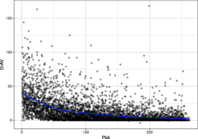
Figure 7-2. Scatterplot with a smoothed, spline trendline for draft pick number against draft approximate value, plotted with ggplot2
Figures 7-1 and 7-2 show that the value of a pick decreases as the pick number increases.
Now, a real question when trying to derive this curve is what are teams looking for when they draft? Are they looking for the average value produced by the pick? Are they looking for the median value produced by the pick? Some other percentile?
The median is likely going to give 0 values for later picks, which is clearly not true since teams trade them all the time, but the mean might also overvalue them because of the hits later in the draft by some teams. Statistically, the median is 0 if more than 50% of picks had 0 value. But the mean can be affected by some really good players who were drafted late. The Patriots, for example, took Tom Brady with the 199th pick in the 2000 draft, and he became one of the best football players of all time. A Business Insider article by Cork Gaines tells the backstory of this pick.
For now, use the mean, but in the exercises you’ll use the median and see if anything changes. “Quantile Regression” provides a brief overview of another type of regression, quantile regression, that might be worth exploring if you want to dive into different model types.
Note
Datasets that contain series (such as daily temperatures or draft picks) often contain both patterns and noise. One way to smooth out this noise is by calculating an average over several sequential observations. This average is often called a rolling average; other names include moving mean, running average, or similar variations with rolling, moving, or running used to describe the mean or average. Key inputs to a rolling average include the window (number of inputs to use), method (such as mean or median), and what to do with the start and end of the series (for example, should the first entries without a full window be dropped or another rule used?).
To smooth out the value for each pick, first calculate the average value for each pick. A couple of the lower picks had NaN values, so replace these values with 0. Then, calculate the six-pick moving mean DrAV surrounding each pick’s average value (that is to say, each DrAV value as well as the 6 before and 6 after, for a window of 13). Also, tell the rolling() function to use min_periods=1 and to center the mean (the rolling average is centered on the current DrAV). Last, groupby() pick and then calculate the average DrAV for each pick position. In Python, use this code:
## Pythondraft_chart_py=draft_py_use_pre2019.groupby(["Pick"]).agg({"DrAV":["mean"]})draft_chart_py.columns=list(map("_".join,draft_chart_py.columns))draft_chart_py.loc[draft_chart_py.DrAV_mean.isnull()]=0draft_chart_py["roll_DrAV"]=(draft_chart_py["DrAV_mean"].rolling(window=13,min_periods=1,center=True).mean())
Tip
For the exercise in Python, you will want to change the rolling()
mean() to be other functions, such as median(), not the groupby()
mean() that is part of the agg().
Then plot the results to create Figure 7-3:
## Pythonsns.scatterplot(draft_chart_py,x="Pick",y="roll_DrAV")plt.show()

Figure 7-3. Scatterplot for draft pick number against draft approximate value (seaborn)
In R, group_by() pick and summarize() with the mean(). Replace NA values with 0. Then use the rollapply() function from the zoo package (make sure you have run library(zoo) and installed the package, since this is the first time you’ve used this package in the book). With rollapply(), use width = 13, and the mean() function (FUN = mean).
Tell the mean() function to ignore NA values with na.rm = TRUE. Fill in missing values with NA, center the mean (so that the rolling average is centered on the current DrAV), and calculate the mean when fewer than 13 observations are present (such as the start and end of the dataframe):
## Rdraft_chart_r<-draft_r_use_pre2019|>group_by(Pick)|>summarize(mean_DrAV=mean(DrAV,na.rm=TRUE))|>mutate(mean_DrAV=ifelse(is.na(mean_DrAV),0,mean_DrAV))|>mutate(roll_DrAV=rollapply(mean_DrAV,width=13,FUN=mean,na.rm=TRUE,fill="extend",partial=TRUE))
Tip
For the exercise in R, you will want to change the rollapply()
mean() to be other functions such as median(), not the group_by()
mean() that is part of summarize().
Then plot to create Figure 7-4:
## Rggplot(draft_chart_r,aes(Pick,roll_DrAV))+geom_point()+geom_smooth()+theme_bw()+ylab("Rolling average (u00B1 6) DrAV")+xlab("Draft pick")
From here, you can simply fit a model to the data to help quantify this result. This model will allow you to use numbers rather than only examining a figure. You can use various models, and some of them (like LOESS curves or GAMs) are beyond the scope of this book. We have you fit a simple linear model to the logarithm of the data, while fixing the y-intercept—and transform back using an exponential function.

Figure 7-4. Scatterplot with smoothed trendline for draft pick number against draft approximate value (ggplot2)
Warning
The log(0) function is mathematically undefined, so people will often add a
value to allow this transformation to occur. Often a small number like
1 or 0.1 is used. Beware: this transformation can change your model
results sometimes, so you may want to try different values for the
number you add.
In Python, first drop the index (so you can access Pick with the model) and then plot:
## Pythondraft_chart_py.reset_index(inplace=True)draft_chart_py["roll_DrAV_log"]=np.log(draft_chart_py["roll_DrAV"]+1)DrAV_pick_fit_py=smf.ols(formula="roll_DrAV_log ~ Pick",data=draft_chart_py).fit()(DrAV_pick_fit_py.summary())
Resulting in:
                            OLS Regression Results
==============================================================================
Dep. Variable:          roll_DrAV_log   R-squared:                       0.970
Model:                            OLS   Adj. R-squared:                  0.970
Method:                 Least Squares   F-statistic:                     8497.
Date:                Sun, 04 Jun 2023   Prob (F-statistic):          1.38e-200
Time:                        09:42:13   Log-Likelihood:                 177.05
No. Observations:                 262   AIC:                            -350.1
Df Residuals:                     260   BIC:                            -343.0
Df Model:                           1
Covariance Type:            nonrobust
==============================================================================
                 coef    std err          t      P>|t|      [0.025      0.975]
------------------------------------------------------------------------------
Intercept      3.4871      0.015    227.712      0.000       3.457       3.517
Pick          -0.0093      0.000    -92.180      0.000      -0.010      -0.009
==============================================================================
Omnibus:                        3.670   Durbin-Watson:                   0.101
Prob(Omnibus):                  0.160   Jarque-Bera (JB):                3.748
Skew:                           0.274   Prob(JB):                        0.154
Kurtosis:                       2.794   Cond. No.                         304.
==============================================================================

Notes:
[1] Standard Errors assume that the covariance matrix of the errors is
    correctly specified.
And then merge back into draft_chart_py and look at the top of the data:
## Pythondraft_chart_py["fitted_DrAV"]=np.exp(DrAV_pick_fit_py.predict())-1draft_chart_py.head()
Resulting in:
   Pick  DrAV_mean  roll_DrAV  roll_DrAV_log  fitted_DrAV
0     1      47.60  38.950000       3.687629    31.386918
1     2      39.85  37.575000       3.652604    31.086948
2     3      44.45  37.883333       3.660566    30.789757
3     4      31.15  36.990000       3.637323    30.495318
4     5      43.65  37.627273       3.653959    30.203606
In R, use the following:
## RDrAV_pick_fit_r<-draft_chart_r|>lm(formula=log(roll_DrAV+1)~Pick)summary(DrAV_pick_fit_r)
Resulting in:
Call:
lm(formula = log(roll_DrAV + 1) ~ Pick, data = draft_chart_r)

Residuals:
     Min       1Q   Median       3Q      Max
-0.32443 -0.07818 -0.02338  0.08797  0.34123

Coefficients:
              Estimate Std. Error t value Pr(>|t|)
(Intercept)  3.4870598  0.0153134  227.71   <2e-16 ***
Pick        -0.0093052  0.0001009  -92.18   <2e-16 ***
---
Signif. codes:  0 '***' 0.001 '**' 0.01 '*' 0.05 '.' 0.1 ' ' 1

Residual standard error: 0.1236 on 260 degrees of freedom
Multiple R-squared:  0.9703,    Adjusted R-squared:  0.9702
F-statistic:  8497 on 1 and 260 DF,  p-value: < 2.2e-16
And then merge back into draft_chart_r and look at the top of the data:
## Rdraft_chart_r<-draft_chart_r|>mutate(fitted_DrAV=pmax(0,exp(predict(DrAV_pick_fit_r))-1))draft_chart_r|>head()
Resulting in:
# A tibble: 6 × 4
   Pick mean_DrAV roll_DrAV fitted_DrAV
  <int>     <dbl>     <dbl>       <dbl>
1     1      47.6      39.0        31.4
2     2      39.8      37.6        31.1
3     3      44.4      37.9        30.8
4     4      31.2      37.0        30.5
5     5      43.6      37.6        30.2
6     6      34.7      37.4        29.9
So, to recap, in this section, you just calculated the estimated value for each pick. Notice that this fit likely underestimates the value of the pick at the very beginning of the draft because of the two-parameter nature of the exponential regression. This can be improved upon with a different model type, like the examples mentioned previously. The shortcomings notwithstanding, this estimate will allow you to explore draft situations, something you’ll do in the very next section.
The Jets/Colts 2018 Trade Evaluated
Now that you have an estimate for the worth of each draft pick, let’s look at what this model would have said about the trade between the Jets and the Colts in Table 7-1:
## Rlibrary(kableExtra)future_pick<-tibble(Pick="Future 2nd round",Value="14.8 (discounted at rate of 25%)")team<-tibble("Receiving team"=c("Jets",rep("Colts",4)))tbl_1<-draft_chart_r|>filter(Pick%in%c(3,6,37,49))|>select(Pick,fitted_DrAV)|>rename(Value=fitted_DrAV)|>mutate(Pick=as.character(Pick),Value=as.character(round(Value,1)))|>bind_rows(future_pick)team|>bind_cols(tbl_1)|>kbl(format="pipe")|>kable_styling()
| Receiving team | Pick | Value |
|---|---|---|
Jets | 3 | 30.8 |
Colts | 6 | 29.9 |
Colts | 37 | 22.2 |
Colts | 49 | 19.7 |
Colts | Future 2nd round | 14.8 (discounted at rate of 25%) |
As you can see, the future pick is discounted at 25% because a rookie contract is four years and the waiting one year is a quarter, or 25%, of the contract for a current year.
Adding up the values from Table 7-1, it looks like the Jets got fleeced, losing an expected 55.6 DrAV in the trade. That’s more than the value of the first-overall pick! These are just the statistically “expected” values from a generic draft pick at that position, using the model developed in this chapter based on previous drafts. Now, as of the writing of this book, what was predicted has come to fruition. You can use new data to see the actual DrAV for the players by creating Table 7-2:
## Rlibrary(kableExtra)future_pick<-tibble(Pick="Future 2nd round",Value="14.8 (discounted at rate of 25)")results_trade<-tibble(Team=c("Jets",rep("Colts",5)),Pick=c(3,6,37,"49-traded for 52","49-traded for 169","52 in 2019"),Player=c("Sam Darnold","Quenton Nelson","Braden Smith","Kemoko Turay","Jordan Wilkins","Rock Ya-Sin"),"DrAV"=c(25,55,32,5,8,11))results_trade|>kbl(format="pipe")|>kable_styling()
| Team | Pick | Player | DrAV |
|---|---|---|---|
Jets | 3 | Sam Darnold | 25 |
Colts | 6 | Quenton Nelson | 55 |
Colts | 37 | Braden Smith | 32 |
Colts | 49—traded for 52 | Kemoko Turay | 5 |
Colts | 49—traded for 169 | Jordan Wilkins | 8 |
Colts | 52 in 2019 | Rock Ya-Sin | 11 |
So, the final tally was Jets 25 DrAV, Colts 111—a loss of 86 DrAV, which is almost three times the first overall pick!
This isn’t always the case when a team trades up to draft a quarterback. For example, the Chiefs traded up for Patrick Mahomes, using two first-round picks and a third-round pick in 2017 to select the signal caller from Texas Tech, and that worked out to the tune of 85 DrAV, and (as of 2022) two Super Bowl championships.
More robust ways to price draft picks, can be found in the sources mentioned in “Analyzing the NFL Draft”. Generally speaking, using market-based data—such as the size of a player’s first contract after their rookie deal—is the industry standard. Pro Football Reference’s DrAV values are a decent proxy but have some issues; namely, they don’t properly account for positional value—a quarterback is much, much more valuable if teams draft that position compared to any other position. For more on draft curves, The Drafting Stage: Creating a Marketplace for NFL Draft Picks (self-published, 2020) by Eric’s former colleague at PFF, Brad Spielberger, and the founder of Over The Cap, Jason Fitzgerald, is a great place to start.
Are Some Teams Better at Drafting Players Than Others?
The question of whether some teams are better at drafting than others is a hard one because of the way in which draft picks are assigned to teams. The best teams choose at the end of each round, and as we’ve seen, the better players are picked before the weaker ones. So we could mistakenly assume that the worst teams are the best drafters, and vice versa. To account for this, we need to adjust expectations for each pick, using the model we created previously. Doing so, and taking the average and standard deviations of the difference between DrAV and fitted_DrAV, and aggregating over the 2000–2019 drafts, we arrive at the following ranking using Python:
## Pythondraft_py_use_pre2019=draft_py_use_pre2019.merge(draft_chart_py[["Pick","fitted_DrAV"]],on="Pick")draft_py_use_pre2019["OE"]=(draft_py_use_pre2019["DrAV"]-draft_py_use_pre2019["fitted_DrAV"])draft_py_use_pre2019.groupby("Tm").agg({"OE":["count","mean","std"]}).reset_index().sort_values([("OE","mean")],ascending=False)
Resulting in:
     Tm    OE
        count      mean        std
26  PIT   161  3.523873  18.878551
11  GNB   180  3.371433  20.063320
8   DAL   160  2.461129  16.620351
1   ATL   148  2.291654  16.124529
21  NOR   131  2.263655  18.036746
22  NWE   176  2.162438  20.822443
13  IND   162  1.852253  15.757658
4   CAR   148  1.842573  16.510813
2   BAL   170  1.721930  16.893993
27  SEA   181  1.480825  16.950089
16  LAC   144  1.393089  14.608528
5   CHI   149  0.672094  16.052031
20  MIN   167  0.544533  13.986365
15  KAN   154  0.501463  15.019527
25  PHI   162  0.472632  15.351785
6   CIN   176  0.466203  15.812953
14  JAX   158  0.182685  13.111672
30  TEN   172  0.128566  12.662670
12  HOU   145 -0.075827  12.978999
28  SFO   184 -0.092089  13.449491
31  WAS   150 -0.450485   9.951758
24  NYJ   137 -0.534640  13.317478
0   ARI   149 -0.601563  14.295335
23  NYG   145 -0.879900  12.471611
29  TAM   153 -0.922181  11.409698
3   BUF   161 -0.985761  12.458855
17  LAR   175 -1.439527  11.985219
19  MIA   151 -1.486282  10.470145
9   DEN   159 -1.491545  12.594449
10  DET   155 -1.765868  12.061696
18  LVR   162 -2.587423  10.217426
7   CLE   170 -3.557266  10.336729
Note
The .reset_index() function in Python helps us because a dataframe in
pandas has row names (an index) that can get confused when appending
values.
Or in R:
## Rdraft_r_use_pre2019<-draft_r_use_pre2019|>left_join(draft_chart_r|>select(Pick,fitted_DrAV),by="Pick")draft_r_use_pre2019|>group_by(Tm)|>summarize(total_picks=n(),DrAV_OE=mean(DrAV-fitted_DrAV,na.rm=TRUE),DrAV_sigma=sd(DrAV-fitted_DrAV,na.rm=TRUE))|>arrange(-DrAV_OE)|>(n=Inf)
Resulting in:
# A tibble: 32 × 4
   Tm    total_picks DrAV_OE DrAV_sigma
   <chr>       <int>   <dbl>      <dbl>
 1 PIT           161  3.52        18.9
 2 GNB           180  3.37        20.1
 3 DAL           160  2.46        16.6
 4 ATL           148  2.29        16.1
 5 NOR           131  2.26        18.0
 6 NWE           176  2.16        20.8
 7 IND           162  1.85        15.8
 8 CAR           148  1.84        16.5
 9 BAL           170  1.72        16.9
10 SEA           181  1.48        17.0
11 LAC           144  1.39        14.6
12 CHI           149  0.672       16.1
13 MIN           167  0.545       14.0
14 KAN           154  0.501       15.0
15 PHI           162  0.473       15.4
16 CIN           176  0.466       15.8
17 JAX           158  0.183       13.1
18 TEN           172  0.129       12.7
19 HOU           145 -0.0758      13.0
20 SFO           184 -0.0921      13.4
21 WAS           150 -0.450        9.95
22 NYJ           137 -0.535       13.3
23 ARI           149 -0.602       14.3
24 NYG           145 -0.880       12.5
25 TAM           153 -0.922       11.4
26 BUF           161 -0.986       12.5
27 LAR           175 -1.44        12.0
28 MIA           151 -1.49        10.5
29 DEN           159 -1.49        12.6
30 DET           155 -1.77        12.1
31 LVR           162 -2.59        10.2
32 CLE           170 -3.56        10.3
To no one’s surprise, some of the storied franchises in the NFL have drafted the best above the draft curve since 2000: the Pittsburgh Steelers, the Green Bay Packers, and the Dallas Cowboys.
It also won’t surprise anyone that last three teams on this list, the Cleveland Browns, the Oakland/Las Vegas Raiders, and the Detroit Lions, all have huge droughts in terms of team success as of the time of this writing. The Raiders haven’t won their division since last playing in the Super Bowl in 2002, the Lions haven’t won theirs since it was called the NFC Central in 1993, and the Cleveland Browns left the league, became the Baltimore Ravens, and came back since their last division title in 1989.
The question is, is this success and futility statistically significant? In Appendix B, we talk about standard errors and credible intervals. One reason we added the standard deviation to this table is so that we could easily compute the standard error for each team. This may be done in Python:
## Pythondraft_py_use_pre2019=draft_py_use_pre2019.merge(draft_chart_py[["Pick","fitted_DrAV"]],on="Pick")draft_py_use_pre2019_tm=(draft_py_use_pre2019.groupby("Tm").agg({"OE":["count","mean","std"]}).reset_index().sort_values([("OE","mean")],ascending=False))draft_py_use_pre2019_tm.columns=list(map("_".join,draft_py_use_pre2019_tm.columns))draft_py_use_pre2019_tm.reset_index(inplace=True)draft_py_use_pre2019_tm["se"]=(draft_py_use_pre2019_tm["OE_std"]/np.sqrt(draft_py_use_pre2019_tm["OE_count"]))draft_py_use_pre2019_tm["lower_bound"]=(draft_py_use_pre2019_tm["OE_mean"]-1.96*draft_py_use_pre2019_tm["se"])draft_py_use_pre2019_tm["upper_bound"]=(draft_py_use_pre2019_tm["OE_mean"]+1.96*draft_py_use_pre2019_tm["se"])(draft_py_use_pre2019_tm)
Resulting in:
    index  Tm_  OE_count  ...        se  lower_bound  upper_bound
0      26  PIT       161  ...  1.487838     0.607710     6.440036
1      11  GNB       180  ...  1.495432     0.440387     6.302479
2       8  DAL       160  ...  1.313954    -0.114221     5.036479
3       1  ATL       148  ...  1.325428    -0.306186     4.889493
4      21  NOR       131  ...  1.575878    -0.825066     5.352375
5      22  NWE       176  ...  1.569551    -0.913882     5.238757
6      13  IND       162  ...  1.238039    -0.574302     4.278809
7       4  CAR       148  ...  1.357180    -0.817501     4.502647
8       2  BAL       170  ...  1.295710    -0.817661     4.261522
9      27  SEA       181  ...  1.259890    -0.988560     3.950210
10     16  LAC       144  ...  1.217377    -0.992970     3.779149
11      5  CHI       149  ...  1.315034    -1.905372     3.249560
12     20  MIN       167  ...  1.082297    -1.576770     2.665836
13     15  KAN       154  ...  1.210308    -1.870740     2.873667
14     25  PHI       162  ...  1.206150    -1.891423     2.836686
15      6  CIN       176  ...  1.191946    -1.870012     2.802417
16     14  JAX       158  ...  1.043109    -1.861808     2.227178
17     30  TEN       172  ...  0.965520    -1.763852     2.020984
18     12  HOU       145  ...  1.077847    -2.188407     2.036754
19     28  SFO       184  ...  0.991510    -2.035448     1.851270
20     31  WAS       150  ...  0.812558    -2.043098     1.142128
21     24  NYJ       137  ...  1.137789    -2.764706     1.695427
22      0  ARI       149  ...  1.171119    -2.896957     1.693831
23     23  NYG       145  ...  1.035711    -2.909893     1.150093
24     29  TAM       153  ...  0.922419    -2.730123     0.885761
25      3  BUF       161  ...  0.981895    -2.910275     0.938754
26     17  LAR       175  ...  0.905997    -3.215282     0.336228
27     19  MIA       151  ...  0.852048    -3.156297     0.183732
28      9  DEN       159  ...  0.998805    -3.449202     0.466113
29     10  DET       155  ...  0.968819    -3.664752     0.133017
30     18  LVR       162  ...  0.802757    -4.160827    -1.014020
31      7  CLE       170  ...  0.792791    -5.111136    -2.003396

[32 rows x 8 columns]
Or in R:
## Rdraft_r_use_pre2019|>group_by(Tm)|>summarize(total_picks=n(),DrAV_OE=mean(DrAV-fitted_DrAV,na.rm=TRUE),DrAV_sigma=sd(DrAV-fitted_DrAV,na.rm=TRUE))|>mutate(se=DrAV_sigma/sqrt(total_picks),lower_bound=DrAV_OE-1.96*se,upper_bound=DrAV_OE+1.96*se)|>arrange(-DrAV_OE)|>(n=Inf)
Resulting in:
# A tibble: 32 × 7
   Tm    total_picks DrAV_OE DrAV_sigma    se lower_bound upper_bound
   <chr>       <int>   <dbl>      <dbl> <dbl>       <dbl>       <dbl>
 1 PIT           161  3.52        18.9  1.49        0.608       6.44
 2 GNB           180  3.37        20.1  1.50        0.440       6.30
 3 DAL           160  2.46        16.6  1.31       -0.114       5.04
 4 ATL           148  2.29        16.1  1.33       -0.306       4.89
 5 NOR           131  2.26        18.0  1.58       -0.825       5.35
 6 NWE           176  2.16        20.8  1.57       -0.914       5.24
 7 IND           162  1.85        15.8  1.24       -0.574       4.28
 8 CAR           148  1.84        16.5  1.36       -0.818       4.50
 9 BAL           170  1.72        16.9  1.30       -0.818       4.26
10 SEA           181  1.48        17.0  1.26       -0.989       3.95
11 LAC           144  1.39        14.6  1.22       -0.993       3.78
12 CHI           149  0.672       16.1  1.32       -1.91        3.25
13 MIN           167  0.545       14.0  1.08       -1.58        2.67
14 KAN           154  0.501       15.0  1.21       -1.87        2.87
15 PHI           162  0.473       15.4  1.21       -1.89        2.84
16 CIN           176  0.466       15.8  1.19       -1.87        2.80
17 JAX           158  0.183       13.1  1.04       -1.86        2.23
18 TEN           172  0.129       12.7  0.966      -1.76        2.02
19 HOU           145 -0.0758      13.0  1.08       -2.19        2.04
20 SFO           184 -0.0921      13.4  0.992      -2.04        1.85
21 WAS           150 -0.450        9.95 0.813      -2.04        1.14
22 NYJ           137 -0.535       13.3  1.14       -2.76        1.70
23 ARI           149 -0.602       14.3  1.17       -2.90        1.69
24 NYG           145 -0.880       12.5  1.04       -2.91        1.15
25 TAM           153 -0.922       11.4  0.922      -2.73        0.886
26 BUF           161 -0.986       12.5  0.982      -2.91        0.939
27 LAR           175 -1.44        12.0  0.906      -3.22        0.336
28 MIA           151 -1.49        10.5  0.852      -3.16        0.184
29 DEN           159 -1.49        12.6  0.999      -3.45        0.466
30 DET           155 -1.77        12.1  0.969      -3.66        0.133
31 LVR           162 -2.59        10.2  0.803      -4.16       -1.01
32 CLE           170 -3.56        10.3  0.793      -5.11       -2.00
Tip
Looking at this long code output, the 95% confidence intervals (CIs) can help
you see which teams’ DrAV_OE differed from 0. In both the Python and
R outputs, 95% CIs are lower_bound and upper_bound.
If this interval does not contain the value, you can consider it
statistically different from 0. If the DrAV_OE is greater than the
interval, the team did statistically better than average. If the
DrAV_OE is less than the interval, the team did statistically worse
than average.
So, using a 95% CI, it looks like two teams are statistically significantly better at drafting players than other teams, pick for pick (the Steelers and Packers), while two teams are statistically significantly worse at drafting players than the other teams (the Raiders and Browns). This is consistent with the research on the topic, which suggests that over a reasonable time interval (such as the average length of a general manager or coach’s career), it’s very hard to discern drafting talent.
The way to “win” the NFL Draft is to make draft pick trades like the Colts did against the Jets and give yourself more bites at the apple, as it were. Timo Riske discusses this more in the PFF article “A New Look at Historical Draft Success for all 32 NFL Teams”.
One place where that famously failed, however, is with one of the two teams that has been historically bad at drafting since 2002, the Oakland/Las Vegas Raiders. In 2018, the Raiders traded their best player, edge player Khalil Mack, to the Chicago Bears for two first-round picks and an exchange of later-round picks. The Raiders were unable to ink a contract extension with Mack, whom the Bears later signed for the richest deal in the history of NFL defensive players. The Sloan Sports Analytics Conference—the most high-profile gathering of sports analytics professionals in the world—lauded the trade for the Raiders, giving that team the award for the best transaction at the 2019 conference.
Generally speaking, trading one player for a bunch of players is going to go well for the team that acquires the bunch of players, even if they are draft picks. However, the Raiders, proven to be statistically notorious for bungling the picks, were unable to do much with the selections, with the best pick of the bunch being running back Josh Jacobs. Jacobs did lead the NFL in rushing yards in 2022, but prior to that point had failed to distinguish himself in the NFL, failing to earn a fifth year on his rookie contract. The other first-round pick in the trade, Damon Arnette, lasted less than two years with the team, while with Mack on the roster, the Bears made the playoffs twice and won a division title in his first year with the club in 2018.
Now, you’ve seen the basics of web scraping. What you do with this data is largely up to you! Like almost anything, the more you web scrape, the better you will become.
Data Science Tools Used in This Chapter
This chapter covered the following topics:
-
Web scraping data in Python and R for the NFL Draft and NFL Scouting Combine data from Pro Football Reference
-
Using
forloops in both Python and R -
Calculating rolling averages in Python with
rolling()and in R withrollapply() -
Reapplying data-wrangling tools you learned in previous chapters
Exercises
-
Change the web-scraping examples to different ranges of years for the NFL Draft. Does an error come up? Why?
-
Use the process laid out in this chapter to scrape NFL Scouting Combine data by using the general URL https://www.pro-football-reference.com/draft/YEAR-combine.htm (you will need to change YEAR). This is a preview for Chapter 8, where you will dive into this data further.
-
With NFL Scouting Combine data, plot the 40-yard dash times for each player, with point color determined by the position the player plays. Which position is the fastest? The slowest? Do the same for the other events. What are the patterns you see?
-
Use the NFL Scouting Combine data in conjunction with the NFL Draft data scraped in this chapter. What is the relationship between where a player is selected in the NFL Draft and their 40-yard dash time? Is this relationship more pronounced for some positions? How does your answer to question 3 influence your approach to this question?
-
For the draft curve exercise, change the six-pick moving average to a six-pick moving median. What happens? Is this preferable?
Suggested Readings
Many books and other resources exist on web scraping. Besides the package documentation for rvest in R and read_html() in pandas, here are two good ones to start with:
-
R Web Scraping Quick Start Guide by Olgun Aydin (Packt Publishing, 2018)
-
Web Scraping with Python, 2nd edition, by Ryan Mitchell (O’Reilly, 2018); 3rd edition forthcoming in 2024
The Drafting Stage: Creating a Marketplace for NFL Draft Picks, referenced previously in this chapter, provides an overview of the NFL Draft along with many great details.