Defining synthetic data

Synthetic data sets and “real” data sets are distinguished by their origins. While real data is collected from measurements of the world (for example, human population data, or users of an application). synthetic data sets are generated using algorithms. These algorithms focus on closely matching the distribution of sensitive real data so that the synthetic data provides similar insights to the real data while also protecting privacy.

Synthetic data sets are particularly valuable in scenarios involving microdata.

Microdata

Microdata is individual level data that “provide[s] information about characteristics of individual people or entities such as households, business enterprises, facilities, farms or even geographical areas such as villages or towns. " ¹

Privatized microdata, which includes individual-level data, cannot be achieved with the techniques introduced in this book so far. Synthetic data sets are a solution for sharing and publishing microdata in a privacy-preserving manner.

In many cases, researchers and data practitioners find that only publishing data estimates can limit analysis and conclusions. Data professionals often need more detailed estimates than the pre-computed summaries provide. Microdata allows you to pick and choose your own variables and create custom estimates.

Sensitive microdata should remain locked within organizations, with limited access to a privileged few. Synthetic data can provide wider access while preserving privacy. This enables exploratory analysis, correlations, and regression without exhausting your privacy budget.

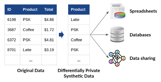
Figure 11-1. Placeholder for Differentially Private Synthetic Data - Image from NIST blog.

Practical Scenarios for Synthetic Data Usage

Synthetic data is a powerful tool for informing practitioners about data distributions and structure. By providing synthetic counterparts that mirror the original data’s statistical properties, SD allows practitioners to understand and familiarize themselves with the data’s characteristics. This understanding aids in developing appropriate methodologies, analyses, and insights.

Eyes-off machine learning refers to situations where the training data is inaccessible to data practitioners, and the machine learning model is trained in a secure computing environment using differentially private learning algorithms. In such cases, validation data can be unavailable or scarce and synthetic data can be an alternative for parameter tuning and feature selection.

Overall, these are the main scenarios where synthetic data sets are valuable:

1. Microdata analysis:

   • Synthetic microdata: privacy protection for individual-level data.

2. General data access:

   • Unlocking data for initial exploration on crucial topics like health, socioeconomic factors and education.

   • Breaking down barriers to data locked within organizations.

   • Enabling wider access to promote inclusivity and foster innovation.

3. Budget-friendly exploratory analysis:

   • Leveraging synthetic data to perform correlations, marginal analyses, and regression.

   • Eliminating the need for significant budget allocation when exploring unknown data territories.

4. Data structure and usage:

   • Synthetic data can play a huge role in informing practitioners about data characteristics.

   • Assisting practitioners in developing appropriate methodologies and analyses.

5. Parameter tuning and feature selection in “eyes-off” machine learning

   • Synthetic data as a valuable resource when validation data is unavailable.

   • Fine-tuning models and selecting relevant features without compromising privacy.

Synthetic Data Generation Algorithms

Synthetic data can be generated using a variety of methods, the choice of which is largely determined by the problem domain and data properties required. These approaches all strive to do the same thing: create a data set with statistical properties similar to a real data set, without directly including data from the real data set. In this section, you will learn about several such approaches, their strengths and weaknesses, and when to use them.

from opendp.smartnoise.synthesizers.mwem import MWEMSynthesizer

# Apply the synthesizer to the data set
synthetic_data = MWEMSynthesizer(Q_count = 400,
                        epsilon = 0.1,
                        iterations = 60,
                        mult_weights_iterations = 40,
                        splits = [],
                        split_factor = 1)
synthetic_data.fit(df.to_numpy())

df_synthesized = pd.DataFrame(synthetic_data.sample(int(df.shape[0])),
                              columns=df.columns)

PrivBayes

PrivBayes was originally proposed as a synthesizer focused on improving the utility of generated synthetic data. This improvement comes by approximating the actual distribution of the data, which is achieved by constructing a Bayesian network using the correlations between the data attributes. PrivBayes can then factorize the joint distribution of the data into marginal distributions. Next, to ensure differential privacy, noise is injected into each of the marginal distributions and the simulated data is sampled from the approximate joint distribution constructed from these noisy marginals.

PrivBayes is particularly powerful when used to generate high-dimensional data. To understand this process fully, let’s first learn what a Bayesian network is.

Bayesian Network

A Bayesian network represents the relationships between multiple random variables. This is typically represented as a directed graph of nodes connected by arrows. If one node points to the other, it means it directly influences the probabilistic outcome.

Consider an example morning routine: you have to leave the house before 8 AM about 50% of the time. So the first node has the table {0.5, 0.5}. If you leave before 8 AM, there is a 75% chance you forget to make coffee. If it is raining, and you have to leave before 8 AM, there is a __ chance you forget to lock the front door. This graphic shows the relationship between the outside factors (time of day, drinking coffee) and the final result that you want to predict - is your front door unlocked?

For any data set with at least 2 attributes, you can measure the correlation between them. For example, a data set with tree ages and heights.

You can calculate the correlation between age and height - for each additional year of age, this type of tree can expect to gain __ meters in height, up to a certain point. More generally, you can construct probabilities that answer the question “given this tree is X years old, what is the probability that it is at least Y meters tall?”

PrivBayes uses a Bayesian network like this to generate joint distributions and then privatizes them via the Laplace mechanism. ³ With these privatized joint distributions in hand, it then generates conditional distributions which are combined to form the final result.

// Pseudo code for PrivBayes

fun noisy_conditionals(D, N, k):
    """
    D: a high-dimensional data set
    N: a Bayesian network
    k: integer
    """

    // Initialize P* - this is the value that will be returned at the end
    p_private = null

    // d is the number of attributes in D
    for i=k+1, i <= d, i++
        // Generate the joint distribution given X and Pi
        Pr[X_i, Pi_i] = generate_joint_distribution(X_i, Pi_i)

        // Privatize the joint distribution using Laplace noise
        Pr_private[X_i, Pi_i] = Pr[X_i, Pi_i] + laplace_noise(4(d-k) / n * epsilon)

        // Set all negative values to 0, and normalize
        normalize_and_set_negative_values_to_zero(Pr_private[X_i, Pi_i])

        // Generate the conditional distribution
        Pr_private[X_i | Pi_i] = generate_conditional(Pr_private[X_i, Pi_i])

        // Add the result to P*, which will be returned at the end
        p_private = p_private + Pr_private[X_i | Pi_i]

    for i=1, i<=k, i++
        Pr_private[X_i | Pi_i] = generate(Pr_private[X_k+1, Pi_k+1])
        p_private = p_private + Pr_private[X_i | Pi_i]

    return p_private

The PrivBayes algorithm is available in the SDGym library. Using the SDGym library, you can generate a synthetic version of the adult data set.

from DataSynthesizer.DataDescriber import DataDescriber
from DataSynthesizer.DataGenerator import DataGenerator
from DataSynthesizer.ModelInspector import ModelInspector
from DataSynthesizer.lib.utils import read_json_file, display_bayesian_network

mode = 'correlated_attribute_mode'
description_file = f'./out/{mode}/{epsilon}/description_{i}.json'
synthetic_data = f'./out/{mode}/{epsilon}/sythetic_data_{i}.csv'
epsilon = 1
# An attribute is categorical if its domain size is less than this threshold.

threshold_value = 20
# specify categorical attributes
categorical_attributes = {'education': True}
# specify which attributes are candidate keys of input dataset.
candidate_keys = {'ids' : True}
# The maximum number of parents in Bayesian network, i.e.
# the maximum number of incoming edges.
degree_of_bayesian_network = 2

# Number of tuples generated in synthetic dataset.
# Here 32561 is the same as input dataset,
# but it can be set to another number.
num_tuples_to_generate = 32561

describer = DataDescriber(category_threshold=threshold_value)
describer.describe_dataset_in_correlated_attribute_mode(
    dataset_file=input_data,
    epsilon=epsilon,
    k=degree_of_bayesian_network,
    attribute_to_is_categorical=categorical_attributes,
    attribute_to_is_candidate_key=candidate_keys)
describer.save_dataset_description_to_file(description_file)
generator = DataGenerator()
generator.generate_dataset_in_correlated_attribute_mode(
    num_tuples_to_generate, description_file)
generator.save_synthetic_data(synthetic_data)

display_bayesian_network(describer.bayesian_network)

================ Constructing Bayesian Network (BN) ================
Adding ROOT marital-status
Adding attribute relationship
Adding attribute workclass
Adding attribute income
Adding attribute education
Adding attribute sex
Adding attribute education-num
Adding attribute capital-gain
Adding attribute occupation
Adding attribute fnlwgt
Adding attribute hours-per-week
Adding attribute capital-loss
Adding attribute age
Adding attribute native-country
Adding attribute race
========================== BN constructed ==========================
Constructed Bayesian network:
    relationship   has parents ['marital-status'].
    workclass      has parents ['relationship', 'marital-status'].
    income         has parents ['workclass', 'relationship'].
    education      has parents ['workclass', 'relationship'].
    sex            has parents ['workclass', 'marital-status'].
    education-num  has parents ['sex', 'education'].
    capital-gain   has parents ['education-num', 'income'].
    occupation     has parents ['education-num', 'income'].
    fnlwgt         has parents ['occupation', 'marital-status'].
    hours-per-week has parents ['income', 'workclass'].
    capital-loss   has parents ['hours-per-week', 'sex'].
    age            has parents ['fnlwgt', 'workclass'].
    native-country has parents ['capital-loss', 'occupation'].
    race           has parents ['fnlwgt', 'sex'].

GANs synthesizer

Since their development in 2014, Generative Adversarial Networks (GAN) have become a powerful tool across a variety of disciplines. Conceptually, a GAN is two interacting machine learning models: a generator, and a discriminator. The generator, true to its name, generates data samples according to some distribution or rules. These data samples are fed to the discriminator along with real data points.

A useful analogy for GANs comes from its originator, Ian Goodfellow. In this rendering, a gan is like a team of counterfitters trying to outsmart the police. ⁴ They continue producing different types of fake currency until the police cannot identify the counterfits. This leads to a scenario where each team is trying to improve at the task they’ve been given: one group wants to make the most convincing fake currency possible, while the other wants to be as accurate as possible when detecting if currency is authentic or not.

Generative Adversarial Network (GAN)

Generative adversarial networks (GANs) are a type of artificial neural network used in machine learning for generating new data samples similar to a given training dataset. They learn patterns and relationships from the input data and then use this knowledge to create new data similar or different from the original dataset. Mathematically, generative adversarial networks are based on a game between two machine learning models, a discriminator model D and the generator model G.

The models play a two-player game to find the minimax of a value function. A minimax strategy examines the worst possible case (maximum loss) and tries to minimize it. Formally, for some function $v$:

In the case of a GAN, the models attempt to minimax the value function $V_0(G,D)$:

Here, $p_z$ is the pre-defined input noise distribution, and $p_d$ is the distribution of the real data X. Here, the goal of the generator is to learn realistic samples that can fool the discriminator, while the goal of the discriminator is to be able to tell generator generated samples from real ones. The solution to the minimax problem leads to a generator whose generated distribution is identical to the distribution of the training dataset.⁵

The discriminator must answer a key question each time: is this real data, or data created by the generator? Thus, a GAN trains the two sub-models to “out-compete” each other according to this metric. When the discriminator is catching most of the generated data and labeling it as fake (sometimes 50% is set as the cutoff point) then training is considered complete. ⁶

Imagine two convolutional neural networks: one generates a 2D array of numbers, while the other tries to determine if a given array is real or fake. This may not sound like much, but if each value in the 2D array represents pixels, then we have the potential for “deepfake” images. While we won’t cover this particular topic in detail here, it serves to highlight the power of GAN as a technique.

Instead, we will focus on using GAN for a more noble purpose: generating synthetic data sets for privacy preservation.

Conditional Tabular GAN (CTGAN)

Conditional Tabular GAN is an approach for generating tabular data. CTGAN is an adaptation of GANs that addresses issues unique to tabular data that conventional GANs cannot handle. These issues include modeling multivariate discrete and mixed discrete and continuous distributions. CTGAN explores discrete samples more evenly via a conditional generator and training-by-sampling. This mode-specific normalization helps to overcome challenges that a traditional GAN faces. Applying differentially private SGD (DP-SGD) in combination with CTGAN yields a DP approach for generating tabular data. This involves adding random noise to the discriminator and clipping the norm to make it differentially private.

from opendp.smartnoise.synthesizers.mwem import MWEMSynthesizer
from opendp.smartnoise.synthesizers.quail import QUAILSynthesizer

from opendp.smartnoise.synthesizers.pytorch.pytorch_synthesizer 
    import PytorchDPSynthesizer
from opendp.smartnoise.synthesizers.preprocessors.preprocessing 
    import GeneralTransformer
from opendp.smartnoise.synthesizers.pytorch.nn.dpctgan import DPCTGAN
from opendp.smartnoise.synthesizers.pytorch.nn.patectgan import PATECTGAN
from diffprivlib.models import LogisticRegression as DPLR
from diffprivlib.models import GaussianNB as DPNB


epsilon = 1.0

synth = PytorchDPSynthesizer(preprocessor=None,
                            gan=DPCTGAN(loss='cross_entropy',
                                        batch_size=1000,
                                        epochs=300,
                                        pack=1,
                                        sigma=5.0,
                                        epsilon=epsilon))



synth.fit(df)
sample_size = df.shape[0]
synthetic = synth.sample(int(sample_size))
# Convert to dataframe
synth_df = pd.DataFrame(synthetic, columns=df.columns)

PATE (Private Aggregation of Teacher Ensembles)

As you saw in Chapter 7, the PATE (Private Aggregation of Teacher Ensembles) framework protects the privacy of sensitive data during training by transferring knowledge from an ensemble of teacher models trained on partitions of the data to a student model. To achieve DP guarantees, only the student model is published while keeping the teachers private. The framework adds Laplacian noise to the aggregated answers from the teachers that are used to train the student models. CTGAN can provide differential privacy by applying the PATE framework. We call this combination PATE-CTGAN, which is similar to PATE-GAN, for images. The original dataset is partitioned into $k$ subsets and a DP teacher discriminator is trained on each subset. Further, instead of using one generator to generate samples, $k$ conditional generators are used for each subset of the data.

Qualified Architecture to Improve Learning

Qualified Architecture to Improve Learning (QUAIL) is an ensemble model approach that combines a DP supervised learning model with a DP synthetic data model to produce DP synthetic data. The QUAIL framework can be used in conjunction with different synthesizer techniques. CTGAN and PATE are the basic methods we utilize in our experiments with the QUAIL ensemble approach. Note that unlike PrivBayes, both the QUAIL-based approaches provide an approximate DP guarantee.

Synthetic data can capture the statistical properties of a data set without containing any real-world data. This means that relationships and trends can be studied without the risk of a privacy violation to anyone whose data is present in the data set. Recent innovations in synthetic data include MWEM and PrivBayes, methods that can efficiently model a real world dataset and privatize the results. These methods are particularly relevant in cases where the data itself cannot be released for legal reasons, but there would still be substantial benefit from studying it.

The type of data you are studying will generally inform the best tool for the job. GANs, for example, can struggle with tabular data, so we have presented the adapted approach of CTGANs for this purpose. Similarly, microdata scenarios may be the initial motivation for choosing a synthetic data approach, and high-dimensional data motivates the need for an approach like PrivBayes. PATE can be helpful in situations where the data cannot cross an institutional barrier - by training teacher models and transferring the knowledge to a public student model, you can learn important patterns from an otherwise inaccessible data set. Now that you have these new tools, you can start constructing robust and powerful DP pipelines: in the next chapter, you’ll learn how to do exactly this.

Potential Problems

There are several common issues you may encounter when generating synthetic data. Some of these may sound familiar if you have worked with machine learning models in the past. The first is a vanishing gradient - this occurs when your generator isn’t providing enough information for the discriminator to proceed with. In essence, your gradient is flat and your model can’t move forward. If this happens, the library should throw an error alerting you.

Another potential problem is failure to converge, which can happen when either the generator or the discriminator starts to dominate the training process. For example, if the generator learns to trick the discriminator quickly, it may be generating low quality data samples and not continuing to improve. Conversely, if the discriminator quickly starts to identify most of the samples correctly, then the generator never learns to produce higher-quality samples. In both cases, the model never converges. The library should also throw an error if convergence isn’t happening quickly enough.

There is one more failure to keep a close eye on, since the library won’t throw an error. This is called mode collapse. When mode collapse happens, the generator is producing data with a single value over and over. This can happen when the generator has learned to reliably trick the discriminator with one well-tailored piece of data. The generator will then send that data point over and over in order to maximize its score. Think back to the term mode from statistics - this is the most frequently-encountered value in a dataset. The name mode collapse refers to the fact that the mode has taken over the entire dataset!

Exercises

1. Run MWEMSynthesizer on the adult data set without preprocessing - what happens?

   1. Preprocess the dataset where each column is categorical with at most 4 keys. Run MWEMSynthesizer again. How is the result different this time?

   2. Evaluate steps 1 and 2 with $ϵ=0.1,1,10$

2. Run DataGenerator on the adult data set with preprocessing - what happens?

   1. Preprocess the dataset where each column is categorical with at most 4 keys. Run DataGenerator again. How is the result different this time?

   2. Evaluate steps 1 and 2 with $ϵ=0.1,1,10$

   3. What are the performance differences between MWEM and PrivBayes before and after preprocessing? Which approach would you reach for first when studying data similar to the adult dataset?

3. Run DPCTGAN on the adult dataset

   1. Preprocess the dataset where each column is categorical with at most 4 keys. Run DPCTGAN again. How is the result different this time?

   2. Evaluate steps 1 and 2 with $ϵ=0.1,1,10$

   3. When does the synthesizer experience mode collapse?