User-level Databases and Event-level Databases

A user-level database is a database where each row in the database represents an individual. For example, the student database from chapter 3 is an example of a user-level database, where each row represents a student.

User-level database

A user-level database is a database where each row corresponds to a unique individual in a database. For such databases, neighboring databases are understood as databases that differ by a single row.

Now suppose there is a database where each row corresponds to a test taken by a student. Since a student can take multiple tests in a year, each student can appear in multiple rows. In this case, each row corresponds to a test rather than a student. Each row uniquely corresponds to an event: a student taking a single test.

Event-level databased

Event-level database is a database where a single individual can contribute multiple events. Usually, each row in the database corresponds to a single event. For this type of database, neighboring databases are understood as databases that differ by a single individual. In event-level databases a single individual can be represented by a fixed number of rows, or by a variable number of rows.

Applying DP to Event-level Databases: A Naive Approach

Given that multiple rows in an event-level database can correspond to a single user, it is reasonable to conclude that user-level and event-level data must be treated differently in order to guarantee differential privacy. Let’s see an example of a differentially private data release that utilizes an event-level database to compute differentially private aggregates. In this example, the employment of differential privacy will follow a naive approach to an event-level problem. This example should help you understand the importance of understanding the nature of the dataset.

Suppose a data scientist wants to release the visit count to four websites. They have access to the following dataset that contains browser logs of 1234 employees of a company, from August to December 2020. Sample of the data:

In this database, each row represents an event described by the following fields:

• Employee Id,

• date of the event,

• time the event occurred, and

• the address of the domain visited.

The data scientist needs to compute a differentially private count of visits to each of the following websites:

• mail.com,

• bank.com,

• social.com,

• games.com

in each of the following months:

• August,

• September,

• October,

• November,

• December

To proceed with the task, the data scientist naively sets the sensitivity of the COUNT query to 1 and starts making queries to the database to get the counts of visits to each website per month.

The data scientist uses the Laplace mechanism to privatize the count. Let’s set the budget of the data release to $ϵ=0.1$.

The data scientist proceeds to make the queries and budget calculations the same way as they would if he had been using a user-level database. If the same budget is spent on each query, each query will require $ϵ=0.005$. The data scientist feels confident this data release will not leak any information about individuals, only overall browsing patterns. The following data is published:

When visit counts are released, the data scientist notices a significant drop in the number of visits from October to November for games.com and social.com. If you knew your co-worker took a leave of absence during this time, then you could surmise your co-worker’s browsing habits, even though the data scientist made a release utilizing the Laplace mechanism, i.e. with noise added.

Could it be a coincidence, or is the data release actually releasing more information than it should about an employee? How did this happen if the data scientist used differential privacy in a data release?

Defining “Neighboring”: Event-level Databases

So far we’ve defined two datasets as neighboring if their distance is 1. However, for event-level datasets, that definition does not apply! We need a more general notion of adjacency to take into account that one individual can affect multiple rows in the data.

Neighboring event-level databases

For two event-level datasets $X$ and $Y$, and distance metric $M$, where $d_M(X,Y)$ is a distance metric relative to M, and an integer k, we say that X and Y are “k-neighboring” provided that $d_M(X,Y)\le k$.

In English, this just says the distance between datasets must be less than k!

from collections import Counter


def d_Sym(u, v):
    """symmetric distance between u and v"""
    # NOT this, as sets are not multisets. Loses multiplicity:
    # return len(set(u).symmetric_difference(set(v)))
    u_counter, v_counter = Counter(u), Counter(v)
    # indirectly compute symmetric difference via the union of asymmetric differences
    return sum(((u_counter - v_counter) + (v_counter - u_counter)).values())

# consider two simple example datasets, u and v
#   [Jane, Joe, John, Jack, Alice]
u = [1,    1,    2,   3,    4]

#   [Jane, Joe, John, Jack] (without Alice!)
v = [1,    1,    2,   3]

# compute the symmetric distance between these two example datasets:
d_Sym(u, v)

Defining Sensitivity: Event-level Databases

In an event-level database, multiple rows may correspond to the actions of a single user. The key is to understand exactly how many rows correspond to each individual.

Let’s say that, in the browser logs example, due to company restrictions, an employee can only make 10 website visits a day. For simplicity, we will consider a dataset consisting of 150 days (5 months). This means that the maximum number of website visits an employee can contribute to the dataset is 1,500. See the exercises at the end of this chapter for more generalizations.

As we’ve already mentioned, the dataset distance is the maximum number of rows that a single user can contribute. It is necessary to consider the dataset distance when calculating the sensitivity.

Sensitivity on event-level databases

For two event-level datasets X and Y that are “k-neighboring”, we say that our function $f$ is $d_{out}$-sensitive with respect to some distance metric $MO$, provided that $d_{MO}(f\left(X\right),f\left(Y\right))\le d_{out}$.

In English, this just says the greatest amount that the function may change is $d_{out}$. This is the same as the definition of sensitivity presented in Chapter 3, but this time we consider datasets $X$ and $Y$ that have a greater distance.

Notice that as $d_{in}$ gets larger, so does $d_{out}$. If the noise scale stays fixed, then this means the privacy guarantee gets weaker as an individual is allowed to contribute more rows. This makes intuitive sense: if an individual contributes more data, then the statistic becomes more sensitive, and the privacy guarantees become looser.

In the browser logs example, the data scientist makes $\mathrm{?????}$ queries.

Given two neighboring databases, $x$ and $y$, the sensitivity of a $\mathrm{?????}$ query (in terms of the L1 distance metric) is given by $ma{x}_{x,y}\parallel \mathrm{?????}\left(x\right)-\mathrm{?????}\left(y\right){\parallel }_1$. Given that the maximum number of website visits an individual may contribute is 4000, the sensitivity of COUNT queries, when applying it to the browser logs database, is 4000.

Now that the data scientist knows that the sensitivity of $\mathrm{?????}$ queries is 4000, they can use the Laplace mechanism, $M_{Lap}$ with the correct parameters for the data release.

The resulting differentially-private data release looks like this:

From the data release, it is hard to know that employee #789 is an outlier when visiting websites. This is what differential privacy should do - mask the presence/absence of any individual in a database.

This example demonstrates how to properly calibrate sensitivity when we know a bound on the distance between neighboring datasets.

What happens when we don’t have a bound on the distance, that is, when the number of events an individual can contribute is unknown or unlimited? In the next example, we will see how to deal with datasets with unknown or unlimited number of events.

Datasets with Unbounded Number of Events per User

When the distance between datasets is unbounded, the sensitivity is also unbounded. We need a finite sensitivity to establish privacy guarantees.

Therefore, in the case of datasets with an unbounded number of events it becomes difficult, or even impossible, to define sensitivity for many functions due to the unbounded number of rows a user might appear in.

Let $k$ be the upper bound on the number of records for a single user in a database. Let $n_i$ be the number of records that a user $u_i$ influences in a database $D$. For each user $u_i$, if $n_i\le k$, the records for user $u_i$ remain the same. If $n_i>k$, we will select $k$ records from all user $u_i$’s records, and discard the remaining $n_i-k$ records.

# to randomly select k items from a stream of items
import random

def reservoir_sampling(stream, k):
    """randomly select k items from stream [0..n-1]"""
    i = 0  # index of events in user event stream[]
    reservoir = [0] * k

    while i < len(stream):
        # Pick a random index from 0 to i.
        j = random.randrange(i+1)

        # If the random value j is smaller than k,
        # replace the element present at the index j
        # with new element from stream
        if j < k:
            reservoir[j] = stream[i]
        i += 1
    return reservoir

Defining the Bound on the Number of Events

The previous section showed how to pre-process an event-level dataset with unbounded number of events and calculate sensitivity for different functions applied to event-level data.

Assume the data scientist has a threshold $b$ already established, and just needs to process the data accordingly. What happens when the data scientist needs to define the threshold $b$?

The choice of threshold $b$ can deeply impact a data analysis. Suppose the data scientist wants to perform an analysis on a database of hospital visits. In this particular database, let’s consider that the data scientist wants to compute the mean number of visits a patient has per year.

The true distribution of the data.

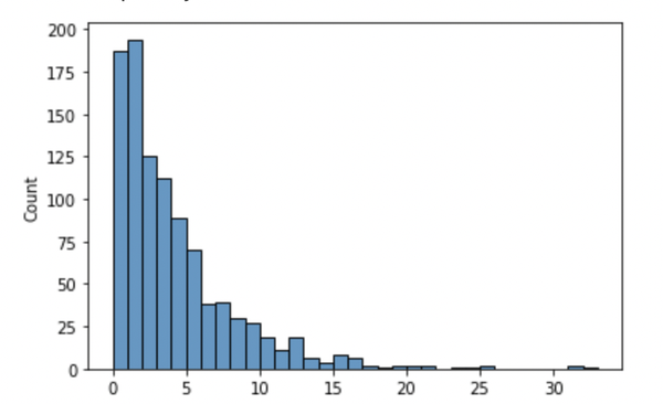
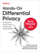
Figure 5-1. Hospital visits per patient without bounding user contribution.

In the original data, without bounding user contribution, the mean number of visits per patient is 2.62 visits, the median is 2 visits, and the total number of visits is 5247. However, we need to set a bound on user contribution so that we can compute the sensitivity of functions we apply to the database. In the original data, the maximum number of visits a patient has is 35. If we decide to make a simple differentially private count query of all visits to the hospital, the sensitivity of the count query is 35. The SmartNoise library can be used to make this query.

import pandas as pd
import snsql

from snsql import Privacy


visits = pd.read_csv('visits.csv')
# This is a filename which will be read in `from_connection`
metadata = 'metadata.yml'

privacy = Privacy(epsilon=1.0)
reader = snsql.from_connection(visits, privacy=privacy, metadata=metadata)

total_visits = reader.execute(
'''
SELECT SUM(visits) as TotalVisits
FROM HospitalRecords.Visits
''')

avg_visits = reader.execute(
'''
SELECT AVG(visits) as AverageVisits
FROM HospitalRecords.Visits
''')

print(total_visits)
[['TotalVisits'], [5275]]
print(avg_visits)
[['AverageVisits'], [2.623022731761945]]

In the case where a data scientist needs to make a decision on the bound k, let’s see the different outcomes between choosing a high versus a low threshold.

Case 1: Low threshold.

Suppose the data scientist chooses a threshold $k$ = 3. A low threshold makes the contribution of each user lower. Instead of the addition or subtraction of a user impacting 33 rows, now it can only impact 3 rows. In the case of $\mathrm{?????}$ queries, by bounding the user contribution to 3 rows, the sensitivity changes from 33 to 3.

The Laplace distribution from which the noise for the $\mathrm{?????}$ mechanism is drawn.

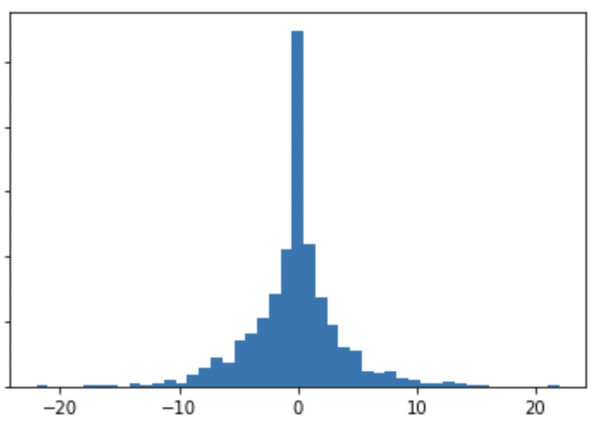
Figure 5-2. Laplace distribution used in differential privacy mechanism for counting hospital visits: bounding user contribution to 3 hospital visits.

Let’s further analyze if it is a good solution to lower the threshold more. The data scientist starts by preprocessing the data, such that each user can have at most 3 hospital visits. The visits from each user are sampled according to some sampling rule, e.g. reservoir sampling. After the data preprocessing, the data has a new distribution.

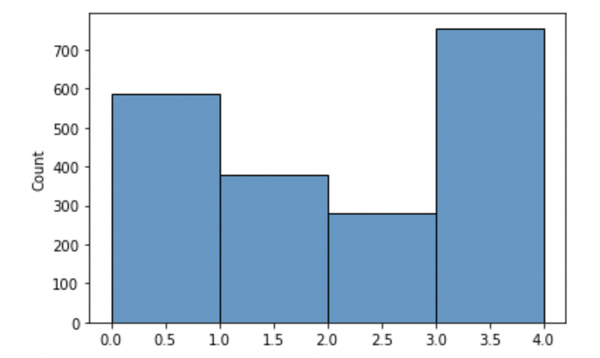
Figure 5-3. Distribution of hospital visits per patient bounding user contribution to 3 hospital visits.

Lowering the bound on the user contribution results in less noise from the Laplace distribution. However, applying this bound can change the data such that the results are compromised. Using the SmartNoise library to make the same queries as before:

import pandas as pd
import snsql

from snsql import Privacy


visits = pd.read_csv('visits.csv')
metadata = 'metadata.yml'

#Calculating the differentially private count of
# all visits and the average number of visits per patient
privacy = Privacy(epsilon=1.0)


reader = snsql.from_connection(visits,
privacy=privacy,
metadata=metadata)


total_visits = reader.execute(
'''
SELECT SUM(Visits) as TotalVisits
FROM HospitalRecords.Visits
''')


avg_visits = reader.execute(
'''
SELECT AVG(Visits) as AverageVisits
FROM HospitalRecords.Visits
''')

print(total_visits)
[['TotalVisits'], [3205]]

print(avg_visits)
[['AverageVisits'], [1.6016713415567314]]

As we can see from the case above, the data scientist set the user contribution threshold too low and changed the data distribution to the point that the results were no longer meaningful.

Let’s see what happens when the threshold is high:

Case 2: High threshold

Now suppose the data scientist chooses a threshold k = 500. A high threshold makes the possible contribution of each user higher. Instead of the addition or subtraction of a user impacting 33 rows, now it can impact up to 500 rows. In the case of COUNT queries, by setting the bound to the user contribution to 500 rows, the sensitivity changes from 33 to 500.

The Laplace distribution from which the noise for the $\mathrm{?????}$ mechanism is drawm.

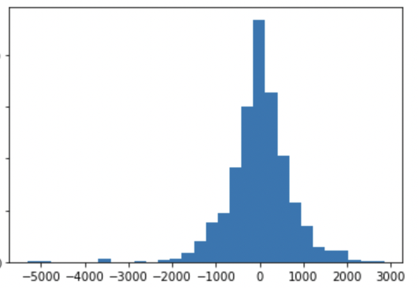
Figure 5-4. Laplace distribution used in differential privacy mechanism for counting hospital visits: bounding user contribution to 500 hospital visits.

The following code uses the SmartNoise library to make the same queries as the previous example. The adjusted sensitivity accounts for up to 500 rows per user:

import pandas as pd
import snsql

from snsql import Privacy


visits = pd.read_csv('visits.csv')
metadata_high = 'metadata_high.yml'

privacy = Privacy(epsilon=1.0)

reader = snsql.from_connection(visits,
privacy=privacy,
metadata=metadata_high)

total_visits = reader.execute(
'''
SELECT SUM(visits) as TotalVisits
FROM HospitalRecords.Visits
''')

avg_visits = reader.execute(
'''
SELECT AVG(visits) as AverageVisits
FROM HospitalRecords.Visits
''')

print(total_visits)
[['TotalVisits'], [4334]]
print(avg_visits)

[['AverageVisits'], [2.254073722721487]]

From these examples we see that the choice of k heavily impacts utility. In many cases, finding an optimal k when the data distribution is unknown might require additional differentially private analyses. We will see more about this in the following section.

Making Queries to a Database of Browser Visits to Top 500 Domains

Consider the example where a data scientist has access to a database with one week of browser logs. The dataset contains over 9000 users and has the following columns:

(This dataset was generated by the authors for educational purposes. The code to generate the dataset can be found in the Hands-on Differential Privacy GitHub. The domains used in this dataset were obtained using Cisco’s DNS list ²)

The data scientist needs to answer the following questions:

• Which are the top 5 most-visited domains?

• How many visits are there to the top 5 domains?

• How many visits are there for each day of the week?

Since the data scientist does not know the optimal k for bounding the number of events, a natural process would be testing different values of k and selecting the best k based on a metric chosen by the data scientist.

Suppose the data scientist wants to find the k that will give the best utility for the counts of visits per user. Doing so in a non-privacy preserving manner would consist in looking at the distribution of events per user and choosing a k that would include 90% or 95% of events.

However, this process is not differentially private. In this case, the data scientist reveals the number of events in the 95th or 90th percentiles.

One way to make the above analysis differentially private is to use part of the privacy budget (we will talk more about this in Chapter 6) to generate a differentially private histogram of the number of events. The data scientist can use a small $ϵ$ and a very large k. Ideally, the k chosen for this analysis should be a value that is much larger than what would be expected as a 95th percentile of k.

For the browsing logs dataset, let’s choose k = 50 visits. To make this preliminary analysis, the data scientist will bound each individual in the dataset to 50 visits.

The data scientist has no information about the data distribution. To make this analysis, instead of generating a histogram of all possible values of number of visits, they will create categories of event ranges.

from importlib.metadata import metadata
import pandas as pd
from snsql import Privacy, from_df
from snsql.sql._mechanisms.base import Mechanism
from snsql.sql.privacy import Stat

budget = 0.5

k = 50
eps = budget/k

metadata = 'events.yaml'
privacy = Privacy(epsilon=eps)
reader = from_df(df, privacy=privacy, metadata=metadata)

query =
'''
SELECT Events, COUNT(Events) AS e
FROM MySchema.MyTable GROUP BY Events
'''


privacy.mechanisms.map[Stat.count] = Mechanism.laplace
print("Running query with Laplace mechanism for count:")
print(privacy.mechanisms.map[Stat.count])
res = reader.execute_df(query)
print(res)

The code returns following output:

Running query with Laplace mechanism for count:
Mechanism.laplace
    Events       e
0   0 - 10  273449
1  10 - 20  118348
2  20 - 30   43548
3  30 - 40   15783
4  40 - 50    5960

Based on this differentially private analysis, $\approx$ 98% of the users have less than 40 events in a week, and $\approx$ 95% of the users have less than 30 events in a week.

But how good are these estimates?

Let’s take a look into the real numbers, and see how close this analysis is to the real values:

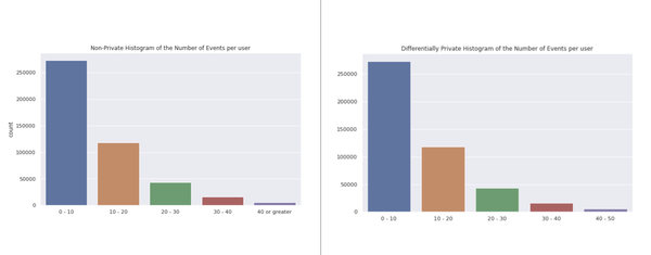
Figure 5-5. Histogram of number of events per user. On the x-axis, number of events (categories). On the y-axis, counts of users that fall into those categories. On the Left, differentially private histogram generated as described above. On the right, histogram with true values.

At first glance, it is easy to notice that the distribution of events per user is very similar. Even though the maximum number of events in the non-private data is greater than 50, choosing 50 as the maximum number of events did not create a bias in the data. The non-private data has 134 as the maximum number of events for a single user.

When looking at quantiles on the non-private data, 92% of users have less than 26 events and 98% of users have less than 40 events. This shows that histogram analysis, even with a small $ϵ$, can give powerful insights when the data distribution is unknown.

Now that the scientist has an understanding of the distribution of events per user in the dataset, they can now sample the events per user.

Using reservoir sampling and k = 40:

import pandas as pd
import numpy as np
import random

k = 40

df= pd.read_csv('data/user_visits.csv')
# Code for generating the user_visits dataset will be available
# at the Hands-on Differential Privacy GitHub


def reservoir_sampling(stream, k):
    """randomly select k items from stream [0..n-1]"""
    i = 0  # index of events in user event stream[]
    reservoir = [0] * k

    while i < len(stream):
        # Pick a random index from 0 to i.
        j = random.randrange(i+1)

        # If the random value j is smaller than k,
        # replace the element present at the index j
        # with new element from stream
        if j < k:
            reservoir[j] = stream[i]
        i += 1
    return reservoir


for i in set(df.ids):
    if len(df[df.ids == i]) <= k:
        continue
    else:
        indexes = list(df[df.ids == i].index)
        sample_ids = reservoir_sampling(indexes, k)
        drop_ids = list(set(indexes) - set(sample_ids))
        df = df.drop(drop_ids)

Now that the data has a bounded number of events per individual, making the following queries to the data should be straightforward, since sensitivity can now be easily calculated:

1- Which are the visited domains?
2- How many visits are there to each domain?
3- Average visits per user for each day of the week?

In the above analysis, the data scientist needs to guarantee that the bound k = 40 is accounted for in the sensitivity of all queries.

In the first query, we are interested in the top 5 most-visited domains. As seen in chapter 4, the exponential mechanism is an $ϵ$-differentially private mechanism that provides the ability to select the best alternative from a discrete set of elements. Here, the “best alternative” is relative to a quality scoring function.

The most visited domains in the dataset can be identified by generating a differentially private histogram with the Laplace Mechanism. Due to the tightly bound L1 distance on a vector-valued count query, this kind of mechanism achieves optimal utility.

In the case of the browser logs event-level database, the L1 distance between two count vectors from adjacent databases is at most 40. When querying the counts of visits to each domain using the SmartNoise sql library, we adjust the epsilon in order to account for the database distance.

1 from importlib.metadata import metadata
2 import pandas as pd
3 from snsql import Privacy, from_df
4 from snsql.sql._mechanisms.base import Mechanism
5 from snsql.sql.privacy import Stat
6 
7 epsilon = 2.0
8 
9 k=40
10 
11 adjusted_eps = epsilon/k
12 
13 metadata = 'domain.yaml'
14 privacy = Privacy(epsilon=epsilon)
15 reader = from_df(df, privacy=privacy, metadata=metadata)
16 
17 query = '''SELECT domain, COUNT(domain) AS DomainVisits
18 FROM MySchema.MyTable
19 GROUP BY domain'''
20 
21 privacy.mechanisms.map[Stat.count] = Mechanism.laplace
22 print("Running query with Laplace mechanism for count:")
23 print(privacy.mechanisms.map[Stat.count])
24 res = reader.execute_df(query)
25 print(res.sort_values(by = 'DomainVisits', ascending = False))

The resulting visit count for each domain is:

Running query with Laplace mechanism for count:
Mechanism.laplace
                             domain  DomainVisits
18                windowsupdate.com          3754
19                   www.google.com          3698
8                     microsoft.com          3667
2                data.microsoft.com          3646
0            api-global.netflix.com          3612
10                      netflix.com          3599
5                        google.com          3590
3         events.data.microsoft.com          3586
4                   ftl.netflix.com          3534
14             prod.ftl.netflix.com          3522
7                          live.com          1078
9               microsoftonline.com          1026
12              partner.netflix.net          1003
15         prod.partner.netflix.net           970
1           ctldl.windowsupdate.com           969
6               ichnaea.netflix.com           957
11                      netflix.net           939
17  settings-win.data.microsoft.com           934
13  preapp.prod.partner.netflix.net           924
16      safebrowsing.googleapis.com           915

Comparing with the non-privatized counts:

windowsupdate.com                  3781
www.google.com                     3698
api-global.netflix.com             3652
netflix.com                        3642
data.microsoft.com                 3639
microsoft.com                      3638
google.com                         3600
events.data.microsoft.com          3599
prod.ftl.netflix.com               3590
ftl.netflix.com                    3571
live.com                           1050
partner.netflix.net                1003
microsoftonline.com                 998
prod.partner.netflix.net            989
ichnaea.netflix.com                 982
ctldl.windowsupdate.com             958
safebrowsing.googleapis.com         951
netflix.net                         933
settings-win.data.microsoft.com     914
preapp.prod.partner.netflix.net     914

Consider that the utility of a count vector is measured as follows: 1) order of the domains, and 2) counts of visits for each domain. From this perspective, the values of Counts of Visits on the differentially private vector are relatively close to the non-private vector. The second observation is regarding ranking order of the domains. The top 2 domains are the same in both rankings, so when analyzing the top 5 domains, there are 4 domains in the intersection of the dp-top5 and non-private top5.

The third query, the average visits per user for each day of the week, is formulated as two distinct queries as follows:

1 from importlib.metadata import metadata
2 import pandas as pd
3 from snsql import Privacy, from_df
4 from snsql.sql._mechanisms.base import Mechanism
5 from snsql.sql.privacy import Stat
6 
7 budget = 2.0
8 k = 40
9 eps = budget/k
10 
11 metadata = 'domain.yaml'
12 privacy = Privacy(epsilon=eps)
13 reader = from_df(df, privacy=privacy, metadata=metadata)
14 
15 query_count_domain = '''SELECT Day_id, COUNT(*) AS DomainVisits
16 FROM MySchema.MyTable
17 GROUP BY Day_id'''
18 
19 
20 query_count_users = '''SELECT Day_id, COUNT(DISTINCT ids_num) AS Users
21 FROM MySchema.MyTable
22 GROUP BY Day_id'''
23 
24 privacy.mechanisms.map[Stat.count] = Mechanism.laplace
25 print("Running query with Laplace mechanism for count:")
26 print(privacy.mechanisms.map[Stat.count])
27 
28 
29 domains_visits = reader.execute_df(query_count_domain)
30 print(domains_visits)
31 
32 user_counts = reader.execute_df(query_count_users)
33 print(user_counts)

The result of the queries above are used as input to the average of visits per user calculation. As seen in previous chapters, a differentially private mean when the total size of the database is unknown results in a function with an undefined sensitivity. The most reliable way to compute means is by making two separate queries: One query for the numerator (total number of visits per day) and one query for the denominator (total number of unique users per day). The calculation of the average becomes a post-processing step of two differentially private functions.

Running query with Laplace mechanism for count:
Mechanism.laplace


      Day_id  DomainVisits
0     Friday        232366
1     Monday        233873
2   Saturday        146003
3     Sunday        145656
4   Thursday        232830
5    Tuesday        232038
6  Wednesday        232574


      Day_id   Users
0     Friday  232381
1     Monday  233867
2   Saturday  146040
3     Sunday  145640
4   Thursday  232746
5    Tuesday  232071
6  Wednesday  232576


Average visits per user per day of the week

Friday        1.230472
Monday        1.233458
Saturday      1.147276
Sunday        1.144335
Thursday      1.232094
Tuesday       1.231370
Wednesday     1.232915

The computation of the mean is a post-processing step. As noted in chapter 3, post-processing of differentially private statistics does not incur in additional privacy losses.

The process described in this example illustrates the steps of a practical differentially private data release. This example shows important phases of a differentially private data release, such as when the data scientist:

1. identifies the browser logs data as an event-level dataset

2. recognizes that the number of events per user is unbounded

3. estimates, in a privacy-preserving manner, a bound k of events per user without previous knowledge on the data distribution

4. pre-processes the database in order to make it ready for a differential privacy analysis

5. makes differentially private queries to the database taking into consideration the necessary code changes to account for multiple events per user

6. evaluates the results of different queries

7. post-processes the results. Budget composition analysis is left as an exercise to the reader.

Unknown Key Set

In the previous example, each row of the browser logs database consists of an event, described by a user visiting a domain on a specific day. From the data description, we know that the data only contains logs of visits to 20 domains. The set of days of the week and domains is well-defined. However, what happens if the database has logs to any set of domains? What if the logs contains logs to URLs or search queries? In this case, even if we apply differential privacy to a data release, just knowing that an event exists in the dataset can reveal the presence or absence of an individual. It is very common for URLs and search queries to contain personally identifiable information (PII). This type of scenario happened in the AOL data release mentioned in the beginning of this chapter.

The idea is to throw away rare items to avoid a privacy-compromising situation such as the AOL release. To determine whether a query should be published or not, the frequency of the query plus some noise should exceed a threshold $\tau$.

The above algorithm only releases real queries. Therefore, it does not satisfy pure differential privacy, with $\delta$ = 0.

Conclusion

It is crucially important to understand the structure of a data set before releasing statistics from it. In this chapter, you’ve seen that there is an important difference between user-level and event-level data. Up until now, you have only seen user-level data, where a user only appears in a single row. With event-level data, this condition is relaxed, and a user can appear in multiple (potentially unlimited) rows.

The presence of an individual across multiple rows has implications for the process of ensuring that a statistic is differentially private. You’ve just seen how to understand sensitivity when this is the case. Trying to perform a DP analysis with your prior assumptions would lead to a privacy leakage. In order to have a well-defined sensitivity, you may need to bound the number of rows that a user can appear in. This hasn’t been an issue until now, since each user has only appeared in one row! This clamping can be accomplished via a handy method called reservoir sampling. With reservoir sampling, you can sample a maximum of k rows for each individual. Knowing that each individual appears a maximum of k times, you now have a data set with a well-defined sensitivity.

Exercises

1 For the following data:

a) Calculate the mean

b) Clip the data on [0, 900.00]. How does the mean change?

c) Clip the data on [0, 100.00]. How does the mean change?

d) Plot the mean versus the clipping bound for values from 1.0 to 1000.0

2 Which of the following datasets are adjacent?

a)

b)

3 Using the browser logs dataset:

a) Demonstrate how the presence of rare events can lead to a privacy violation.

b) Set an appropriate value of $\tau$ and demonstrate how this helps preserve privacy

4 Use the browser logs dataset to demonstrate the parallel composability theorem.

a) How do you have to divide the dataset so that it is disjoint?

b) How does this process differ from using parallel composition on a user-level dataset?