Automated Machine Learning: An Overview

Automated machine learning (AutoML) is an umbrella-term for the various processes and tools that automates parts of the machine learning process. On a high level, AutoML refers to any algorithms and methodologies that seek to solve one or more of the following problems:

Data preprocessing

Machine learning requires data, and raw data can come from various sources and in different formats. To make raw data useful, human experts typically have to comb over the data, normalize values, remove erroneous or corrupted data, and ensure data consistency.

Feature engineering

Training models with too few input variables (or “features”) can lead to inaccurate models. However, too many features can also be problematic - the learning process would slower and more resource-consuming, and overfitting problems can occur. Coming up with the right set of features can be the most time-consuming part of building a machine learning model. Automated feature engineering can speed up the process of feature extraction, selection, and transformation.

Model selection

Once you have all the training data, you need to pick the right training model for your dataset. The ideal model should be as simple as possible while still providing a good measure of prediction accuracy.

Hyperparameter tuning

Most learning models have a number of parameters that are external to the model, such as the learning rate, batch size, and the number of layers in the neural network. We call these “hyperparameters” to distinguish them from model parameters that are adjusted by the learning process. Hyperparameter tuning is the process of automating the search process for these parameters, in order to improve the accuracy of the model.

Neural architecture search

A related field to hyperparameter tuning is neural architecture search (NAS). Instead of choosing between a fixed range of values for each hyperparameter value, NAS seeks to take automation one step further and generate an entire neural network that outperforms hand-crafted architectures. Common methodologies for NAS include reinforcement learning and evolutionary algorithms.

The focus of this chapter will be on the latter two problems—hyperparameter tuning and neural architecture search. These two fields are closely related and can be solved using similar methodologies.

Hyperparameter Tuning with Kubeflow Katib

In Chapter 7, it was mentioned that we needed to set a few hyperparameters. In machine learning, hyperparameters refer to parameters that are set before the training process begins (as opposed to model parameters which are learned from the training process). Examples of hyperparameters include the learning rate, number of decision trees, number of layers in a neural network, etc.

The concept of hyperparameter optimization is very simple: select the set of hyperparameter values that lead to optimal model performance. A hyperparameter tuning framework is a tool that does exactly that. Typically, the user of such a tool would define a few things:

• The list of hyperparameters and their valid range of values (called the “search space”)

• The metrics used to measure model performance

• The methodology to use for the searching process

Kubeflow comes packaged with Katib ², a general framework for hyperparameter tuning. Among similar open-source tools, Katib has a few distinguishing features:

Kubernetes-native

This means that Katib experiments can be ported wherever Kubernetes runs.

Multi-framework support

Katib supports many popular learning frameworks, with first-class support for TensorFlow and PyTorch distributed training.

Language agnostic

Training code can be written in any language, as long as it is built as a Docker image.

In this chapter, we’ll take a look at how Katib simplifies hyperparameter optimization.

Katib Concepts

Let’s begin by defining a few terms that are central to the workflow of Katib (as illustrated in Figure 10-1):

Experiment

An experiment is an end-to-end process that takes a problem (e.g., tuning a training model for handwriting recognition), an objective metric (maximize the prediction accuracy), and a search space (range for hyperparameters), and produces a final set of optimal hyperparameter values.

Suggestion

A suggestion is one possible solution to the problem we are trying to solve. Since we are trying to find the combination of hyperparameter values that lead to optimal model performance, a suggestion would be one set of hyperparameter values from the specified search space.

Trial

A trial is one iteration of the experiment. Each trial takes a suggestion and executes a worker process (packaged through Docker) that produces evaluation metrics. Katib’s controller then computes the next suggestion based on previous metrics and spawns new trials.

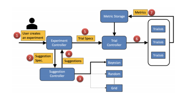
Figure 10-1. Katib system workflow (https://arxiv.org/pdf/2006.02085.pdf)

Another important aspect of hyperparameter tuning is how to find the next set of parameters. As of the time of this writing, Katib supports the following search algorithms:

Grid search

Also known as a parameter sweep, Grid Search is the simplest approach—exhaustively search through possible parameter values in the specified search space. Although resource-intensive, Grid Search has the advantage of having high parallelism since the tasks are completely independent.

Random search

Similar to grid search, the tasks in random search are completely independent. Instead of enumerating every possible value, random search attempts to generate parameter values through random selection. When there are many hyperparameters to tune (but only a few have significant impact on model performance), random search can vastly outperform Grid Search. Random search can be useful when the number of discrete parameters is high, which makes grid search infeasible.

Bayesian optimization

This is a powerful approach that uses probability and statistics to seek better parameters. Bayesian optimization builds a probabilistic model for the objective function, finds parameter values that perform well on the model, then iteratively updates the model based on metrics collected during trial runs. Intuitively speaking, Bayesian optimization seeks to improve upon a model by making informed guesses. This optimization method relies on previous iterations to find new parameters, and can be parallelized. While trials are not as independent as grid or random search, Bayesian optimization can find results with less trials overall.

Hyperband

This is a relative new approach that selects configuration values randomly. But unlike traditional random search, Hyperband only evaluates each trial for a small number of iterations. Then it takes the best performing configurations and runs them longer, repeating this process until a desired result is reached. Due to its similarity to random search, tasks can be highly parallelized.

Other experimental algorithms

Such as Tree of Parzen Estimators (TPE) and Covariance Matrix Adaptation Evolution Strategy (CMA-ES), both implemented by using the Goptuna optimization framework.

One final piece of the puzzle in Katib is the metrics collector. This is the process that collects and parses evaluation metrics after each trial and pushes them into the persistent database. Katib implements metrics collection through a sidecar container, which runs alongside the main container in a pod.

Overall, Katib’s design makes it highly scalable, portable, and extensible. Since it is part of the Kubeflow platform, Katib natively supports integration with many of Kubeflow’s other training components, like the TFJob and PyTorch operators. Katib is also the first hyperparameter tuning framework that supports multitenancy, making it ideal for a cloud hosted environment.

Installing Katib

Katib is installed by default. To install Katib as a standalone service, you can use the following script in the GitHub repo:

git clone https://github.com/kubeflow/katib
bash ./katib/scripts/v1beta1/deploy.sh

If your Kubernetes cluster doesn’t support dynamic volume provisioning, you would also create a persistent volume:

pv_path=https://raw.githubusercontent.com/kubeflow/katib/master/manifests
/v1beta1/pv/pv.yaml
kubectl apply -f pv_path

After installing Katib components, you can navigate to the Katib dashboard to verify that it is running. If you installed Katib through Kubeflow and have an endpoint, simply navigate to the Kubeflow dashboard and select “Katib” in the menu. Otherwise, you can set up port forwarding to test your deployment:

kubectl port-forward svc/katib-ui -n kubeflow 8080:80

Then navigate to:

http://localhost:8080/katib/

Running Your First Katib Experiment

Now that Katib is up and running in your cluster, let’s take a look at how to run an actual experiment. In this section we will use Katib to tune a simple MNist model. You can find the source code and all configuration files on Katib’s GitHub page here: https://github.com/kubeflow/katib/tree/master/examples/v1beta1/mxnet-mnist.

python mnist.py --batch_size=100 --learning_rate=0.1

metrics_name=metrics_value

apiVersion: "kubeflow.org/v1beta1"
kind: Experiment
metadata:
  namespace: kubeflow
  labels:
    controller-tools.k8s.io: "1.0"
  name: random-example
spec:
  objective:               
    type: maximize
    goal: 0.99
    objectiveMetricName: Validation-accuracy
    additionalMetricNames:
      - Train-accuracy
  algorithm:               
    algorithmName: random
  parallelTrialCount: 3    
  maxTrialCount: 12
  maxFailedTrialCount: 3
  parameters:              
    - name: --lr
      parameterType: double
      feasibleSpace:
        min: "0.01"
        max: "0.03"
    - name: --num-layers
      parameterType: int
      feasibleSpace:
        min: "2"
        max: "5"
    - name: --optimizer
      parameterType: categorical
      feasibleSpace:
        list:
        - sgd
        - adam
        - ftrl
  trialTemplate:           
    goTemplate:
        rawTemplate: |-
          apiVersion: batch/v1
          kind: Job
          metadata:
            name: {{.Trial}}
            namespace: {{.NameSpace}}
          spec:
            template:
              spec:
                containers:
                - name: {{.Trial}}
                  image: docker.io/kubeflowkatib/mxnet-mnist
                  command:
                  - "python3"
                  - "/opt/mxnet-mnist/mnist.py"
                  - "--batch-size=64"
                  {{- with .HyperParameters}}
                  {{- range .}}
                  - "{{.Name}}={{.Value}}"
                  {{- end}}
                  {{- end}}
                restartPolicy: Never

    image: docker.io/kubeflowkatib/mxnet-mnist
    command:
      - "python3"
      - "/opt/mxnet-mnist/mnist.py"
      - "--batch-size=64"

kubectl apply -f random-example.yaml

kubectl -n kubeflow describe experiment random-example

Name:         random-example
Namespace:    kubeflow
Labels:       controller-tools.k8s.io=1.0
Annotations:  <none>
API Version:  kubeflow.org/v1beta1
Kind:         Experiment
Metadata:
  Creation Timestamp:  2019-12-22T22:53:25Z
  Finalizers:
    update-prometheus-metrics
  Generation:        2
  Resource Version:  720692
  Self Link:         /apis/kubeflow.org/v1beta1/namespaces/kubeflow/experiments/random-example
  UID:               dc6bc15a-250d-11ea-8cae-42010a80010f
Spec:
  Algorithm:
    Algorithm Name:        random
    Algorithm Settings:    <nil>
  Max Failed Trial Count:  3
  Max Trial Count:         12
  Metrics Collector Spec:
    Collector:
      Kind:  StdOut
  Objective:
    Additional Metric Names:
      accuracy
    Goal:                   0.99
    Objective Metric Name:  Validation-accuracy
    Type:                   maximize
  Parallel Trial Count:     3
  Parameters:
    Feasible Space:
      Max:           0.03
      Min:           0.01
    Name:            --lr
    Parameter Type:  double
    Feasible Space:
      Max:           5
      Min:           2
    Name:            --num-layers
    Parameter Type:  int
    Feasible Space:
      List:
        sgd
        adam
        ftrl
    Name:            --optimizer
    Parameter Type:  categorical
  Trial Template:
    Go Template:
      Raw Template:  apiVersion: batch/v1
kind: Job
metadata:
  name: {{.Trial}}
  namespace: {{.NameSpace}}
spec:
  template:
    spec:
      containers:
      - name: {{.Trial}}
        image: docker.io/kubeflowkatib/mxnet-mnist-example
        command:
        - "python"
        - "/mxnet/example/image-classification/train_mnist.py"
        - "--batch-size=64"
        {{- with .HyperParameters}}
        {{- range .}}
        - "{{.Name}}={{.Value}}"
        {{- end}}
        {{- end}}
      restartPolicy: Never
Status:                                       
  Conditions:
    Last Transition Time:  2019-12-22T22:53:25Z
    Last Update Time:      2019-12-22T22:53:25Z
    Message:               Experiment is created
    Reason:                ExperimentCreated
    Status:                True
    Type:                  Created
    Last Transition Time:  2019-12-22T22:55:10Z
    Last Update Time:      2019-12-22T22:55:10Z
    Message:               Experiment is running
    Reason:                ExperimentRunning
    Status:                True
    Type:                  Running
  Current Optimal Trial:                      
    Observation:
      Metrics:
        Name:   Validation-accuracy
        Value:  0.981091
    Parameter Assignments:
      Name:          --lr
      Value:         0.025139701133432946
      Name:          --num-layers
      Value:         4
      Name:          --optimizer
      Value:         sgd
  Start Time:        2019-12-22T22:53:25Z
  Trials:            12                       
  Trials Running:    2
  Trials Succeeded:  10
Events:              <none>

Katib User Interface

Alternatively, you can use Katib’s user interface to submit and monitor your experiments. If you have a Kubeflow deployment, you can navigate to the Katib UI by clicking on “Katib” in the navigation panel and then “Hyperparameter Tuning” on the following screen (see Figure 10-2).

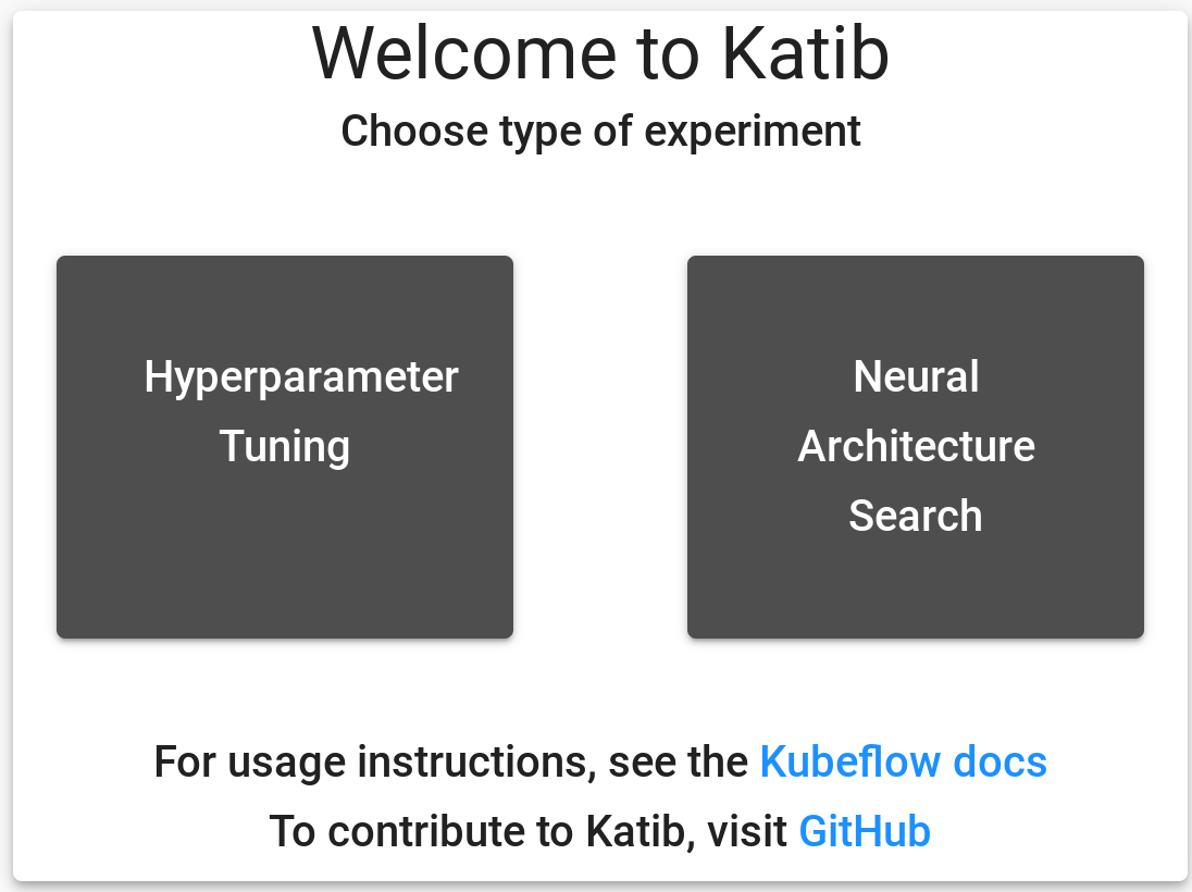
Figure 10-2. Katib UI main page

Let’s submit our random search experiment here (see Figure 10-3). You can simply paste a YAML in the textbox here, or have one generated for you by following the UI. To do this, click on the Parameters tab.

Figure 10-3. Configuring a new experiment, part 1

You should see a panel like Figure 10-4. Enter the necessary configuration parameters on this page—define a run budget and the validation metrics.

Figure 10-4. Configuring a new experiment, part 2

Then scroll down the page and finish up the rest of the experiment, by configuring the search space and the trial template. For the latter, you can just leave it on the default template. When you are done, click “Deploy.”

Now that the experiment is running, you can monitor its status and see a visual graph of the progress (see Figure 10-5). You can see your running and completed experiments by navigating to the drop-down menu in the Katib dashboard, and then selecting “UI” and then “Monitor.”

Figure 10-5. Katib UI for an experiment

Below this graph (Figure 10-6), you can see a detailed breakdown of each trial, the values of the hyperparameters for each trial, and the final metric values. This is very useful for comparing the effects of certain hyperparameters on the model performance.

Figure 10-6. Katib metrics for an experiment

Since we are also collecting validation metrics along the way, we can actually plot the graph for each trial. Click a row to see how the model performs with the given hyperparameter values across time (Figure 10-7):

Figure 10-7. Metrics for each trial

Tuning Distributed Training Jobs

In Chapter 7 we have seen an example of using Kubeflow to orchestrate distributed training. What if we want to use Katib to tune parameters for a distributed training job?

The good news is that Katib natively supports integration with TensorFlow and PyTorch distributed training. A MNist example with TensorFlow can be found from Katib’s GitHub page. This example uses the same MNist distributed training example we’ve seen in Chapter 7, and directly integrates it into the Katib framework. In the example, we will launch an experiment to tune hyperparameters (learning rate and batch size) for a distributed TensorFlow job.

apiVersion: "kubeflow.org/v1beta1"
kind: Experiment
metadata:
  namespace: kubeflow
  name: tfjob-example
spec:
  parallelTrialCount: 3             
  maxTrialCount: 12
  maxFailedTrialCount: 3
  objective:                        
    type: maximize
    goal: 0.99
    objectiveMetricName: accuracy_1
  algorithm:
    algorithmName: random
  metricsCollectorSpec:             
    source:
      fileSystemPath:
        path: /train
        kind: Directory
    collector:
      kind: TensorFlowEvent
  parameters:                       
    - name: learning_rate
      parameterType: double
      feasibleSpace:
        min: "0.01"
        max: "0.05"
    - name: batch_size
      parameterType: int
      feasibleSpace:
        min: "100"
        max: "200"
  trialTemplate:
    trialParameters:
      - name: learningRate
        description: Learning rate for the training model
        reference: learning_rate
      - name: batchSize
        description: Batch Size
        reference: batch_size
    trialSpec:
      apiVersion: "kubeflow.org/v1"
      kind: TFJob
      spec:
        tfReplicaSpecs:             
          Worker:
            replicas: 2
            restartPolicy: OnFailure
            template:
              spec:
                containers:
                  - name: tensorflow
                    image: gcr.io/kubeflow-ci/tf-mnist-with-summaries:1.0
                    imagePullPolicy: Always
                    command:
                      - "python"
                      - "/var/tf_mnist/mnist_with_summaries.py"
                      - "--log_dir=/train/metrics"
                      - "--learning_rate=${trialParameters.learningRate}"
                      - "--batch_size=${trialParameters.batchSize}"

So now you have learned how to use Katib to tune hyperparameters. But notice that you still have to select the model yourself. Can we reduce the amount of human work even further? What about other subfields in AutoML? In the next section we will look at how Katib supports the generation of entire artificial neural networks.

Neural architecture search

Neural architecture search (NAS) is a growing sub-field in automated machine learning. Unlike hyperparameter tuning, where the model is already chosen and our goal is the optimize its performance by turning a few knobs, in NAS we are trying to generate the network architecture itself. Recent research has shown that NAS can outperform handcrafted neural networks on tasks like image classification, object detection, and semantic segmentation.³

Most the methodologies for NAS can be categorized as either generation methods or mutation methods. In generation methods, the algorithm will propose one or more candidate architectures in each iteration. These proposed architectures are then evaluated and then refined in the next iteration. In mutation methods, an overly-complex architecture is proposed first, and subsequent iterations will attempt to prune the model.

Katib currently supports two implementations of NAS: “Differentiable Architecture Search (DARTS),”⁴, and “Efficient Neural Architecture Search (ENAS).”⁵ DARTS achieves scalability of NAS by relaxing the search space to be continuous instead of discrete, and utilizes gradient descent to optimize the architecture. ENAS takes a different approach, by observing that in most NAS algorithms the bottleneck occurs during the training of each child model. ENAS forces each child model to share parameters, thus improving the overall efficiency.

The general workflow of NAS in Katib is similar to hyperparameter search, with an additional step for constructing the model architecture. An internal module of Katib, called the Model Manager, is responsible for taking topological configurations and mutation parameters, and constructing new models. Katib then uses the same concepts of trials and metrics to evaluate the model’s performance.

As an example, this is the spec of a NAS experiment using DARTS:

apiVersion: "kubeflow.org/v1beta1"
kind: Experiment
metadata:
  namespace: kubeflow
  name: darts-example-gpu
spec:
  parallelTrialCount: 1
  maxTrialCount: 1
  maxFailedTrialCount: 1
  objective:
    type: maximize
    objectiveMetricName: Best-Genotype
  metricsCollectorSpec:
    collector:
      kind: StdOut
    source:
      filter:
        metricsFormat:
          - "([\w-]+)=(Genotype.*)"
  algorithm:
    algorithmName: darts
    algorithmSettings:
      - name: num_epochs
        value: "3"
  nasConfig:                     
    graphConfig:
      numLayers: 3
    operations:
      - operationType: separable_convolution
        parameters:
          - name: filter_size
            parameterType: categorical
            feasibleSpace:
              list:
                - "3"
      - operationType: dilated_convolution
        parameters:
          - name: filter_size
            parameterType: categorical
            feasibleSpace:
              list:
                - "3"
                - "5"
      - operationType: avg_pooling
        parameters:
          - name: filter_size
            parameterType: categorical
            feasibleSpace:
              list:
                - "3"
      - operationType: max_pooling
        parameters:
          - name: filter_size
            parameterType: categorical
            feasibleSpace:
              list:
                - "3"
      - operationType: skip_connection
  trialTemplate:
    trialParameters:
      - name: algorithmSettings
        description: Algorithm settings of DARTS Experiment
        reference: algorithm-settings
      - name: searchSpace
        description: Search Space of DARTS Experiment
        reference: search-space
      - name: numberLayers
        description: Number of Neural Network layers
        reference: num-layers
    trialSpec:
      apiVersion: batch/v1
      kind: Job
      spec:
        template:
          spec:
            containers:
              - name: training-container
                image: docker.io/kubeflowkatib/darts-cnn-cifar10
                imagePullPolicy: Always
                command:
                  - python3
                  - run_trial.py
                  - --algorithm-settings="${trialParameters.algorithmSettings}"
                  - --search-space="${trialParameters.searchSpace}"
                  - --num-layers="${trialParameters.numberLayers}"
                resources:
                  limits:
                    nvidia.com/gpu: 1
            restartPolicy: Never

Advantages of Katib Over Other Frameworks

There are many similar open-source systems for hyperparameter search, among them are NNI, Optuna, Ray Tune, and HyperOpt. In addition, the original design of Katib was inspired by Google Vizier. These frameworks offer many capabilities similar to Katib, namely the ability to configure parallel hyperparameter sweeps using a variety of algorithms, there are a few features of Katib that makes it unique:

Design catering to both user and admin.

Most tuning frameworks are designed to cater to the user - the data scientist performing the tuning experiment. Katib is also designed to make life easier for the system admin, who is responsible for maintaining the infrastructure, allocating compute resources, and monitoring system health.

Cloud native design

Other frameworks (such as Ray Tune) may support integration with Kubernetes, but often requires additional effort to set up a cluster. By contrast, Katib is the first hyperparameter search framework to base its design entirely on Kubernetes - every one of its resources can be accessed and manipulated by Kubernetes APIs.

Scalable and portable

Because Katib uses Kubernetes as its orchestration engine, it is very easy to scale up an experiment. You can run the same experiments on a laptop for prototyping and deploy the job to a production cluster with minimal changes to the spec. By contrast, other frameworks require additional effort to install and configure depending on the hardware availability.

Extensible

Katib offers flexible and pluggable interfaces for its search algorithms and storage systems. Most other frameworks come with a preset list of algorithms and have hardcoded mechanisms for metrics collection. In Katib, the user can easily implement a custom search algorithm and integrate it with the framework.

Native support

For advanced features like distributed training and neural archiecture search.

Conclusion

In this chapter we’ve taken a quick overview of automated machine learning (AutoML), and learned how it can accelerate the development of machine learning models by automating time-consuming tasks like hyperparameter search. With techniques like automated hyperparameter tuning, you can scale up the development of your models while sustaining high model quality.

We’ve then used Katib—a Kubernetes-native tuning service from the Kubeflow platform, to configure and execute a hyperparameter search experiment. We’ve also shown how you can use Katib’s dashboard to submit, track, and visualize your experiments.

We’ve also explored how Katib handles Neural Architecture Search (NAS). Katib currently supports two methods of NAS—DARTS and ENAS, with more development to follow.

Hopefully this has given you some insights into how Katib can be leveraged to reduce the amount of work in your machine learning workflows. Katib is still an evolving project, and you can follow the latest developments on Katib’s GitHub page.

Thank you for joining us on your adventures in learning Kubeflow. We hope that Kubeflow meets your needs and helps you delivery on the promise of machine learning value to your organization. To keep up to date on the latest changes with Kubeflow we encourage you to subscribe to join the Kubeflow Slack and mailing lists.