Chapter 6. Artifact and Metadata Store
Machine learning typically involves dealing with a large amount of raw and intermediate (transformed) data where the ultimate goal is creating and deploying the model. In order to understand our model it is necessary to be able to explore data sets used for its creation and transformations (data lineage). The collection of these data sets and transformation applied to them is called the metadata of our model. 1
Model metadata is critical for reproducibility in machine learning; reproducibility is critical for reliable production deployments. Capturing the metadata allows us to understand variations when rerunning jobs or experiments. Understanding variations is necessary to iteratively develop and improve our models. It also provides a solid foundation for model’s comparison. As Pete Warden defined in this post:
To reproduce results, code, training data, and the overall platform need to be recorded accurately.
The same information is also required for other common ML operations—model comparison, reproducible model creation, etc.
There are many different options for tracking the metadata of models. Kubeflow has a built in tool called Kubeflow ML Metadata2 for this. The goal of the tool is to help Kubeflow users to understand and manage their machine learning (ML) workflows by tracking and managing the metadata that the workflows produce. Other tools for tracking metadata that we can integrate into our Kubeflow pipelines is ML Flow Tracking. It provides API and UI for logging parameters, code versions, metrics, and output files when running your machine learning code and for later visualizing the results.
In this chapter we will discuss capabilities of Kubeflow’s ML Metadata project and show how it can be used. We will also consider shortcomings of this implementation and explore usage of additional third party software— MLflow. 3
Kubeflow Metadata
Kubeflow Metadata is a library for recording and retrieving metadata associated with model creation. In the current implementation, Kubeflow Metadata provides only Python APIs. To use other languages, you need to implement the language specific Python plugin to be able to use the library. To understand how it works, we will start with a simple artificial example showing the basic capabilities of Kubeflow Metadata using a very simple notebook (based on this demo).4
Implementation of Kubeflow Metadata starts with required imports (Example 6-1):
Example 6-1. Required imports
fromkfmdimportmetadataimportpandasfromdatetimeimportdatetime
In Kubeflow Metadata all the information is organized in terms of a workspace, run and execution. You need to define a workspace (Example 6-2) so Kubeflow can track and organize the records. The code below shows how this can be done
Example 6-2. Define a workspace
ws1=metadata.Workspace(# Connect to metadata-service in namespace kubeflow.backend_url_prefix="metadata-service.kubeflow.svc.cluster.local:8080",name="ws1",description="a workspace for testing",labels={"n1":"v1"})r=metadata.Run(workspace=ws1,name="run-"+datetime.utcnow().isoformat("T"),description="a run in ws_1",)exec=metadata.Execution(name="execution"+datetime.utcnow().isoformat("T"),workspace=ws1,run=r,description="execution example",)
Tip
Workspace, Run and execution can be defined multiple times in the same or different applications. If they do not exist, they will be created, if they already exist, they will be used.
Kubeflow does not automatically track the data sets used by the application. They have to be explicitly registered in code. Following a classic MNIST example data sets registration in Metadata should be implemented as following:
Example 6-3. Metadata example
data_set=exec.log_input(metadata.DataSet(description="an example data",name="mytable-dump",owner="[email protected]",uri="file://path/to/dataset",version="v1.0.0",query="SELECT * FROM mytable"))
In addition to data, Kubeflow Metadata allows to store information about created Model and its metrics. The code implementing it is presented below:
Example 6-4. Metadata Example 2
model=exec.log_output(metadata.Model(name="MNIST",description="model to recognize handwritten digits",owner="[email protected]",uri="gcs://my-bucket/mnist",model_type="neural network",training_framework={"name":"tensorflow","version":"v1.0"},hyperparameters={"learning_rate":0.5,"layers":[10,3,1],"early_stop":True},version="v0.0.1",labels={"mylabel":"l1"}))metrics=exec.log_output(metadata.Metrics(name="MNIST-evaluation",description="validating the MNIST model to recognize handwritten digits",owner="[email protected]",uri="gcs://my-bucket/mnist-eval.csv",data_set_id=data_set.id,model_id=model.id,metrics_type=metadata.Metrics.VALIDATION,values={"accuracy":0.95},labels={"mylabel":"l1"}))
The combination of the above code snippets implement all of the main steps of storing model creation metadata:
-
Defining workspace, run and execution
-
Store information about data assets used for model creation
-
Store information about the created model, including its version, type, training framework and hyperparameters used for its creation.
-
Store information about model evaluation metrics.
In real world implementations they should be used in the actual code to capture metadata used for data preparation, machine learning, etc. See Chapter 7 for examples of what, where, and how this information is captured.
Collecting metadata is useful only if there are ways to view it. Kubeflow Metadata provides two ways of viewing it—programmatically and using Metadata UI.
Programmatic Query
The following functionality is available for programmatic query.
First, we list all the models in the workspace:
Example 6-5. List all models
pandas.DataFrame.from_dict(ws1.list(metadata.Model.ARTIFACT_TYPE_NAME))
In our code we created only a single model, which is returned as a result of this query (see Figure 6-1).

Figure 6-1. List of models
Next, we get basic lineage. In our case we created a single model, so, the returned lineage will contain only ID of this model.
Example 6-6. Basic lineage
("model id is"+model.id)

returns:
model id is 2
Then we find the execution that produces this model. In our toy application we created a single execution. An ID of this execution is returned as a result of this query.
Example 6-7. Find the execution
output_events=ws1.client.list_events2(model.id).eventsexecution_id=output_events[0].execution_id(execution_id)
Returns
1.
Finally, we find all events related to that execution:
Example 6-8. Getting all related events
all_events=ws1.client.list_events(execution_id).eventsassertlen(all_events)==3("All events related to this model:")pandas.DataFrame.from_dict([e.to_dict()foreinall_events])
In our case we used a single input which was used to create a model and metrics. As a result, the result of this query looks as shown in Figure 6-2.
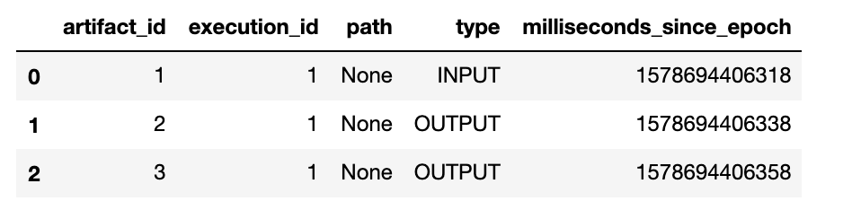
Figure 6-2. Query result as table
Kubeflow Metadata UI
In addition to providing APIs for writing code to analyze metadata, Kubeflow Metadata tool provides a UI, which allows you to view metadata without writing code. Access to Metadata UI is done through the main Kubeflow UI, as seen in Figure 6-3.
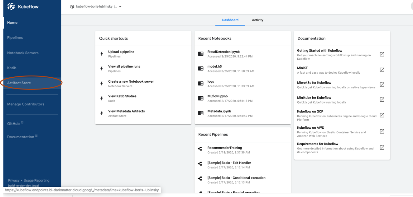
Figure 6-3. Accessing metadata UI
Once you click on Artifact Store you should see the list of available artifacts (logged metadata events), as in Figure 6-4.
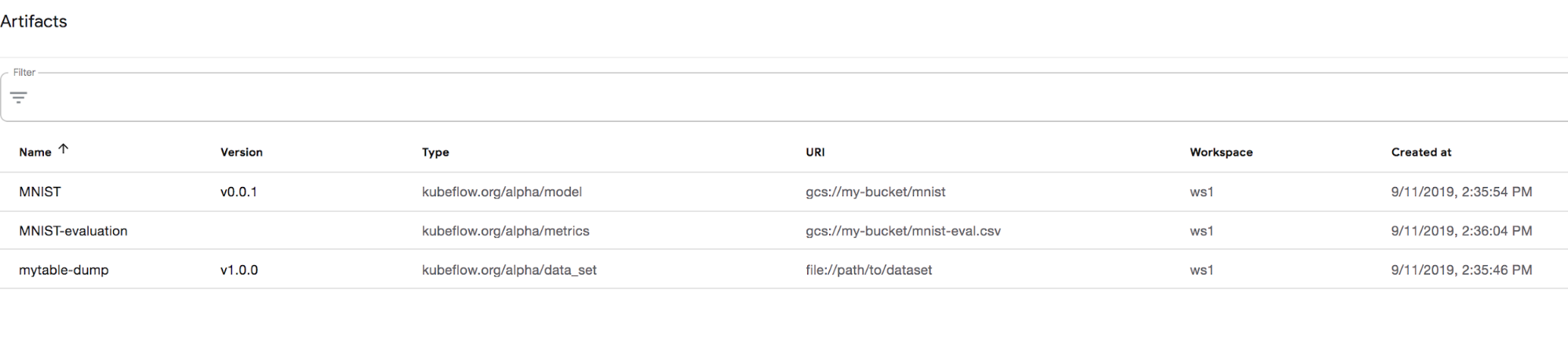
Figure 6-4. List of artifacts in Artifact Store UI
From this view we can click on the individual artifact and see its details, as shown in Figure 6-5.
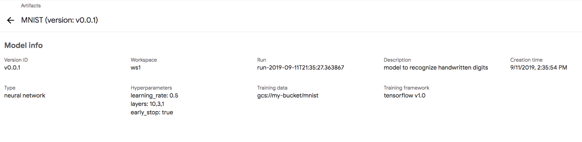
Figure 6-5. Artifact view
Kubeflow Metadata provides some basic capabilities for storing and viewing of machine learning metadata, its capabilities however are extremely limited, especially in terms of viewing and manipulating stored metadata. A more powerful implementation of machine learning metadata management is implemented by MLflow. Although mlflow is not part of Kubeflow distribution, it’s very easy to deploy it alongside Kubeflow and use it from Kubeflow based applications, as described below.
Using MLflow’s Metadata Tools with Kubeflow
MLflow is an open source platform for managing the end-to-end machine learning life cycle. It includes three primary functions:
-
Tracking experiments to record and compare parameters and results (MLflow Tracking).
-
Packaging ML code in a reusable, reproducible form in order to share with other data scientists or transfer to production (MLflow Projects).
-
Managing and deploying models from a variety of ML libraries to a variety of model serving and inference platforms (MLflow Models).
For the purposes of our Kubeflow metadata discussion we will only discuss deployment and usage of MLflow tracking components—an API and UI for logging parameters, code versions, metrics, and output files when running your machine learning code and for later visualizing the results. MLflow Tracking lets you log and query experiments using Python, REST, R, and Java APIs, which significantly extends the reach of APIs, allowing to store and access metadata from different ML components.
MLflow Tracking is organized around the concept of runs, which are executions of some piece of data science code. Each run records the following information:
-
Code Version. Git commit hash used for the run, if it was run from an MLflow Project.
-
Start and End Time. Start and end time of the run
-
Source. Name of the file to launch the run, or the project name and entry point for the run if run from an MLflow Project.
-
Parameters. Key-value input parameters of your choice. Both keys and values are strings.
-
Metrics. Key-value metrics, where the value is numeric. Each metric can be updated throughout the course of the run (for example, to track how your model’s loss function is converging), and MLflow records and lets you visualize the metric’s full history.
-
Artifacts. Output files in any format. For example, you can record images (for example, PNGs), models (for example, a pickled scikit-learn model), and data files (for example, a Parquet file) as artifacts.
Most of the MLflow examples use local MLflow installations, which is not appropriate for our purposes. For our implementation we need a cluster based installation allowing us to write metadata from different docker instances and view them centrally. Following the approach outlined in the project MLFLow Tracking Server based on Docker and AWS S3, the overall architecture of such MLflow tracking component deployment is presented in Figure 6-6.
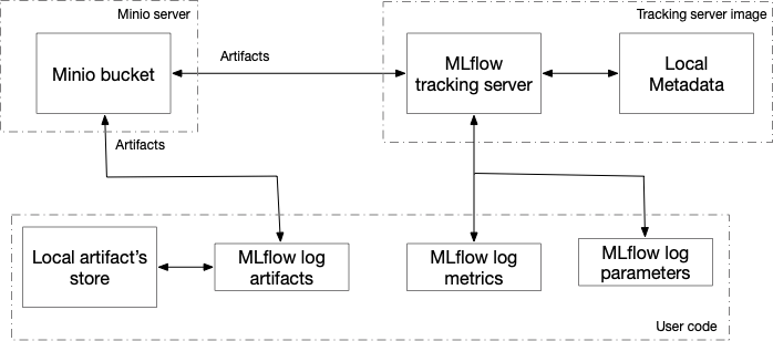
Figure 6-6. Overall architecture of MLflow components deployment
The main components of this architecture are:
-
Minio server, already part of the Kubeflow installation
-
MLflow tracking server—MLflow UI component—an additional component that needs to be added to Kubeflow installation to support MLflow usage.
-
User code, such as notebook, Python, R, or Java application.
Creating and Deploying an MLflow Tracking Server
MLflow tracking server allows you to record MLflow runs to local files, to a SQLAlchemy compatible database, or remotely to a tracking server. In our implementation we are using a remote server.
An MLflow tracking server has two components for storage: a backend store and an artifact store.The backend store is where MLflow Tracking Server stores experiment and run metadata as well as parameters, metrics, and tags for runs. MLflow supports two types of backend stores: file store and database-backed store. For simplicity we will be using a file store. In our deployment, this file store is part of the docker image, which means that this data is lost in the case of server restart. If you need longer term storage, you can either use an external file system, like NFS server, or a database. The artifact store is a location suitable for large data (such as an S3 bucket or shared NFS file system) and is where clients log their artifact output (for example, models). To make our deployment cloud independent, we decided to use Minio (part of Kubeflow) as an artifact store. Based on these decisions, a docker file for building of the MLflow tracking server look like follows (similar to implementation here).
Example 6-9. MLFlow tracking server
FROMpython:3.7RUNpip3 install --upgrade pip&&pip3 install mlflow --upgrade&&pip3 install awscli --upgrade&&pip3 install boto3 --upgradeENVPORT 5000ENVAWS_BUCKET bucketENVAWS_ACCESS_KEY_ID aws_idENVAWS_SECRET_ACCESS_KEY aws_keyENVFILE_DIR /tmp/mlflowRUNmkdir -p /opt/mlflow COPY run.sh /opt/mlflowRUNchmod -R777/opt/mlflow/ENTRYPOINT["/opt/mlflow/run.sh"]
Here we first load MLflow code (using PIP), set environment variables, and then copy and run the startup script. The startup script used here looks like Example 6-10.5
Example 6-10. MLFlow startup script
#!/bin/shmkdir -p$FILE_DIRmlflow server--backend-store-uri file://$FILE_DIR--default-artifact-root s3://$AWS_BUCKET/mlflow/artifacts--host 0.0.0.0--port$PORT
This script sets an environment and then verifies that all required environment variables are set. Once validation succeeds, an MLflow server is started. Once the docker is created the following Helm command (the Helm chart is located on GitHub.) can be used to install the server
helm install <location of the Helm chart>
This Helm chart installs three main components implementing the MLflow tracking server:
- Deployment
-
Deploying MLflow server itself (single replica). The important parameters here are the environment, including minio endpoint, credentials, and bucket used for artifact storage.
- Service
-
Creating a kubernetes service exposing MLflow deployment.
- Virtual service
-
Exposing MLflow service to users through the Istio ingress gateway used by Kubeflow.
Once the server is deployed, we can get access to the UI, but at this point it will say that there are no available experiments. Let’s now look at how this server can be used to capture metadata.6
Logging Data on Runs
As an example of logging data, let’s look at simple code below.7 We will start by installing required packages:
Example 6-11. Install Required
!pipinstallpandas--upgrade--user!pipinstallmlflow--upgrade--user!pipinstalljoblib--upgrade--user!pipinstallnumpy--upgrade--user!pipinstallscipy--upgrade--user!pipinstallscikit-learn--upgrade--user!pipinstallboto3--upgrade--user
Here mlflow and boto3 are the packages required for metadata logging, while the rest are used for machine learning itself. Once these packages are installed, we can define required imports:
Example 6-12. Import required libraries
importtimeimportjsonimportosfromjoblibimportParallel,delayedimportpandasaspdimportnumpyasnpimportscipyfromsklearn.model_selectionimporttrain_test_split,KFoldfromsklearn.metricsimportmean_squared_error,mean_absolute_error,r2_score,explained_variance_scorefromsklearn.exceptionsimportConvergenceWarningimportmlflowimportmlflow.sklearnfrommlflow.trackingimportMlflowClient
Here again, os and the last three imports are required for mlflow logging, while the rest are used for machine learning. Now we need to define environment variables required for proper access to Minio server for storing artifacts:
Example 6-13. Set Environment Variables
os.environ['MLFLOW_S3_ENDPOINT_URL']='http://minio-service.kubeflow.svc.cluster.local:9000'os.environ['AWS_ACCESS_KEY_ID']='minio'os.environ['AWS_SECRET_ACCESS_KEY']='minio123'
Note here that in addition to the tracking server itself MLFLOW_S3_ENDPOINT_URL is defined not only in the tracking server definition, but also in the code, that actually captures the metadata. This is because, as we mentioned above, user code writes to the artifact store directly, bypassing the server.
Here we skip the majority of the code (the full code can be found at GitHub) and concentrate only on the parts related to the MLflow logging. The next step is connecting to the tracking server and creating an experiment:
Example 6-14. Create Experiment
remote_server_uri="http://mlflowserver.kubeflow.svc.cluster.local:5000"mlflow.set_tracking_uri(remote_server_uri)experiment_name="electricityconsumption-forecast"mlflow.set_experiment(experiment_name)
Once connected to the server and creating (choosing) an experiment, we can start logging data. As an example let’s look at the code for storing KNN regressor information.
Example 6-15. Sample KNN model
deftrain_knnmodel(parameters,inputs,tags,log=False):withmlflow.start_run(nested=True):……………………………………………….# Build the modeltic=time.time()model=KNeighborsRegressor(parameters["nbr_neighbors"],weights=parameters["weight_method"])model.fit(array_inputs_train,array_output_train)duration_training=time.time()-tic# Make the predictiontic1=time.time()prediction=model.predict(array_inputs_test)duration_prediction=time.time()-tic1# Evaluate the model predictionmetrics=evaluation_model(array_output_test,prediction)# Log in mlflow (parameter)mlflow.log_params(parameters)# Log in mlflow (metrics)metrics["duration_training"]=duration_trainingmetrics["duration_prediction"]=duration_predictionmlflow.log_metrics(metrics)# log in mlflow (model)mlflow.sklearn.log_model(model,f"model")# Save model#mlflow.sklearn.save_model(model, f"mlruns/1/{uri}/artifacts/model/sklearnmodel")# Tag the modelmlflow.set_tags(tags)
In this code snippet, we can see how different kinds of data about model creation and prediction test statistics is logged. The information here is very similar to the information captured by Kubeflow Metadata and includes inputs, models, and metrics.
Finally, similar to Kubeflow Metadata, MLflow allows you to access this metadata programmatically. The main APIs provided by MLflow include:
Example 6-16. Getting the the runs for a given experiment
df_runs=mlflow.search_runs(experiment_ids="0")("Number of runs done :",len(df_runs))df_runs.sort_values(["metrics.rmse"],ascending=True,inplace=True)df_runs.head()
Getting the the runs for a given experiment

Sorting runs based on the specific parameters
MLFlow will sort runs by Root Mean Square Error (rmse) and show the best ones.
For additional capabilities of the programmatic runs querying consult the MLflow documentation.
With all the capabilities of running programmatic queries, the most powerful way to evaluate runs’ metadata is through MLflow UI, which we will cover next.
Using MLflow UI
The Tracking UI in MLflow lets you visualize, search and compare runs, as well as download run artifacts or metadata for analysis in other tools. Because MLflow is not part of the Kubeflow its access is not provided by Kubeflow UI. Based on the provided Virtual service, MLflow UI is available at <Kubeflow Istio ingress gateway URL>/mlflow[].
Figure 6-7 shows the results produced by the run described.
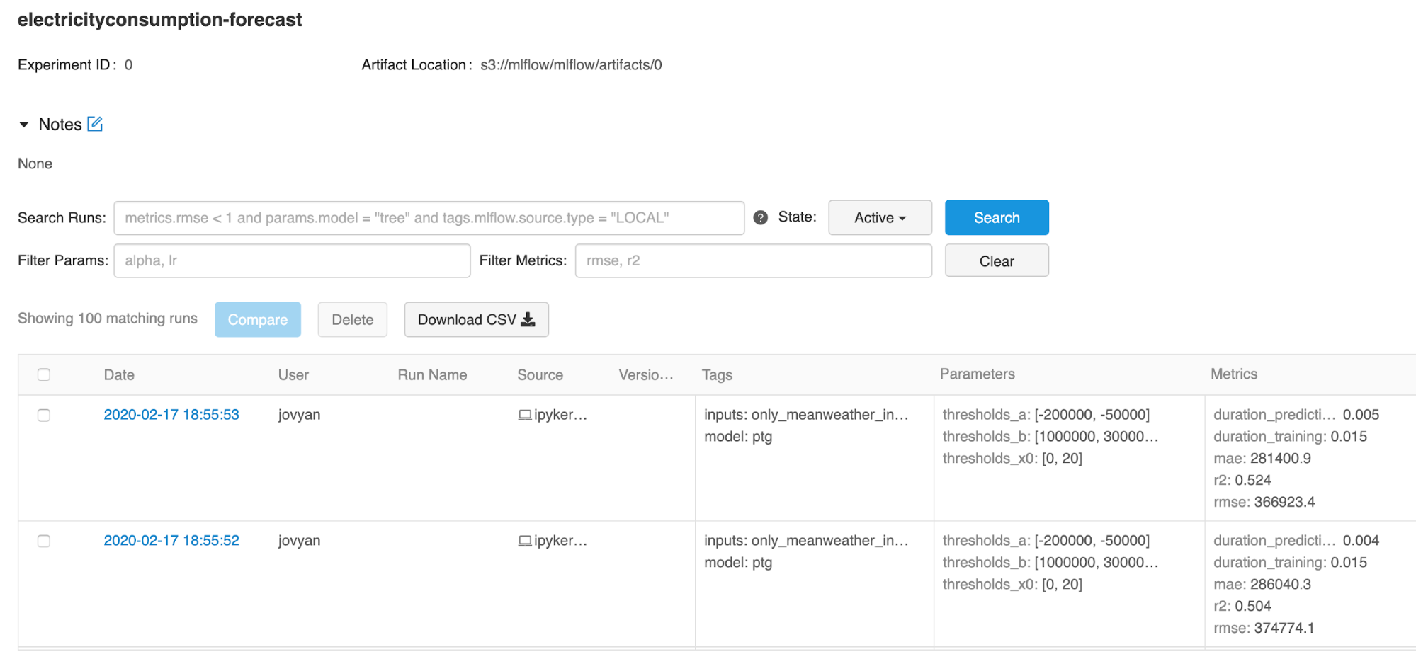
Figure 6-7. MLflow main page
It is possible to filter results using the search box. For example, if we want to see only results for the KNN model, then the search criteria tags.model="knn” can be used. You can also use more complex filters, such as tags.model="knn” and metrics.duration_prediction < 0.002, which will return results for the KNN model for which prediction duration is less than 0.002 sec. By clicking on the individual run we can see its details, as shown in Figure 6-8.
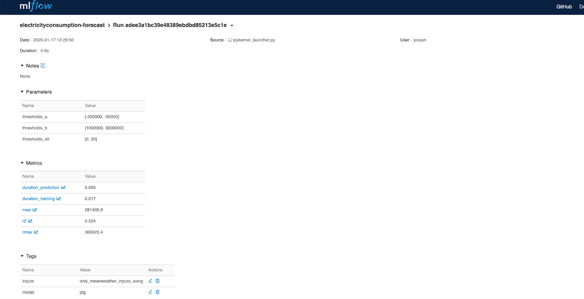
Figure 6-8. View of the individual run
Alternatively, we can compare several runs by picking several runs and click compare, as seen in Figure 6-9.

Figure 6-9. Run comparison view
We can also view metrics comparison for multiple runs, as seen in Figure 6-10.8
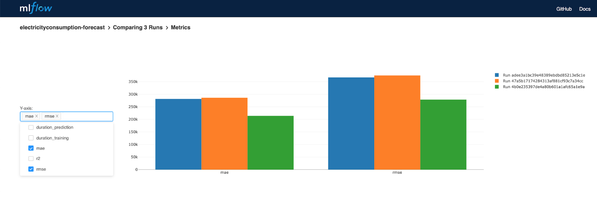
Figure 6-10. Run metrics comparison view
Conclusion
In this chapter we have shown how the Kubeflow Metadata component of the Kubeflow deployment supports storing and viewing of ML metadata. We have also discussed shortcomings of this implementation, including its Python-only support and weak UI, among others. Lastly, we have covered how to supplement Kubeflow with additional components with the similar functionality—MLflow and additional capabilities that can be achieved in this case.
In the next chapter, we’ll explore using Kubeflow in conjunction with TensorFlow to train and serve models.
1 For a good background on metadata for machine learning and an overview of what to capture refer to this blog post.
2 Note that Kubeflow ML metadata is different from ML Metadata. which is part of TFX
3 MLFlow was initially developed by DataBricks and currently is part of Linux Foundation.
4 The complete code for this notebook is located in github
5 This is a simplified implementation. For complete implementation, see GitHub.
6 Here we are showing usage of Python APIs. For additional APIs (R, Java, Rest) refer to MLflow documentation.
7 The code is adopted from this article.
8 Also see tracking-ui documentation for additional UI capabilities.