Chapter 9. Machine Learning in BigQuery
Artificial intelligence (AI) is the domain of computer science focused on building computational systems that are capable of acting autonomously. Over the years, many different subfields have arisen in AI, but an approach that has proven successful in recent years has been the idea of using large datasets to train general-purpose models (such as decision trees and neural networks) that can solve complex problems with great accuracy.
Teaching a computer based on examples is called supervised machine learning, and it can be carried out in BigQuery with the data remaining in place. In this chapter, we look at how to solve a wide variety of machine learning problems using BigQuery ML. Even though machine learning can be carried out in BigQuery, being able to use powerful, industry-standard machine learning frameworks such as TensorFlow on the data in BigQuery can give us access to a much wider variety of machine learning models and components. Hence, in this chapter we also look at the connections that exist between BigQuery and full-fledged machine learning frameworks.
What Is Machine Learning?
If we have collected historical data (and what is a data warehouse for, if not precisely this?), and the historical data contains the correct answers (called the “label”), we can train machine learning models on this data to predict the outcome for cases where the label is not yet known. For example, if we have a historical dataset of actual sales figures, we can train machine learning models to predict sales in the future. As with data analytics, machine learning in BigQuery is also carried out in SQL.
Formulating a Machine Learning Problem
For example, suppose that your business operates several hundred movie theaters all over the country, and you want to predict how many movie tickets will sell for a particular showtime at a particular theater—this sort of prediction is useful if you are trying to determine how to schedule movies. If you have data about the movies that have been run in the past, our machine learning problem might be formulated as follows: use data about the movies in our historical dataset to learn the number of tickets sold for each showtime in each theater. Then apply that machine learning model to a candidate movie to determine how much demand there will be for this movie at a specific showtime.
The attributes of the movie that you will use as inputs to the machine learning model are called the features of the model. The label is what you want to learn how to predict, and in this case, the label is the number of tickets sold. Following are some examples of features that you might want to include in your model:
-
Motion picture content rating1 (for example, PG-13 means that parental guidance is recommended for children younger than 13)
-
Is the showtime on a workday or on a weekend/holiday?
-
At what time of day is the show (afternoon, evening, or night)?
-
Movie genre (comedy, thriller, etc.)
-
How long ago was the movie released (in days)?
-
Average critics’ rating of the movie (scale of 1 to 10)
-
Total box office receipts for the previous movie by this director, if applicable
-
Total box office receipts for the previous movie by the lead actor, if applicable
-
Theater location
-
Theater type (e.g., multiplex, drive-in, mall, etc.)
Note that the title of the movie, as is, is not a good input to the machine learning model.2 Though Tinker Tailor Soldier Spy, a 2011 movie, might be part of our training dataset, we will typically not be interested in predicting the performance of that exact movie (for one, it has already run in our theater). Instead, our interest will be in predicting the performance of, say, Deep Water Horizon, another thriller with similar critical reviews that was released in 2016.
Hence, the machine learning model needs to be based on features of the movie (things that describe the movie), not things that uniquely identify it. This way, our model might guess that Deep Water Horizon, if run at similar timings to Tinker Tailor Soldier Spy, will perform similarly because the movies are in the same genre, and because the critics’ rating of the movies are similar.
The first four features (rating, type of showtime, showtime, genre) are categorical features, by which we mean that they take one of a finite number of possible values. In BigQuery, any feature that is a string is considered a categorical feature. If the database representation of categorical features happens to be some other type (for example, the showtime might be a number such as 1430 or a timestamp), you should cast it as a string in your query. The next four features (time since release, critics’ ratings, box office receipts for director and lead actor) are numeric features, by which we mean that they are numbers with meaningful magnitudes. The last two features (theater type and location) will need to be represented in special ways; we discuss choices later in this chapter.
The label, or the correct answer for the prediction problem, is given by the number of tickets sold historically. During the training of the machine learning model, BigQuery is shown the input features and corresponding labels and creates the model that captures this information (see Figure 9-1). Then, during prediction, the trained machine learning model can be applied on a new set of input features to gain an estimate of how many tickets we can expect to sell if we schedule the movie at a specific time and location.

Figure 9-1. During training, the model is shown features and their corresponding labels. Then the trained model can be used for prediction. Given a set of features, the model predicts a value for the label.
Types of Machine Learning Problems
We tend to use different machine learning models and techniques depending on the nature of the input features and the labels. In this subsection, we’ll provide brief definitions of the types of problems. We cover the solutions to these problems in greater detail in the rest of this chapter.
Classification
If the label is a categorical variable, the type of machine learning problem is called classification. The output of a classification model is the probability that a row belongs to a label value. For example, if you were to train a machine learning model to predict whether a show will sell out, you would be using a classification model, and the output of the model would be the probability that a show sells out.
Many classification problems have two classes: the show sells out or it doesn’t, a customer buys the item or they don’t, the flight is late or it isn’t. These are called binary classification problems. In such cases, the label column should be True or False, or it should be 1 or 0. The prediction from the model will be the probability that the label is True. We typically threshold the probability at 0.5 to determine the most likely class.
A classification problem can have multiple classes. For example, revisiting our bike rental scenario, you might want to predict the station at which a bicycle will be returned, and because there are hundreds of possible values for this categorical label, this is a multiclass classification problem. The output of such a machine learning model will be a set of probabilities, one for each station in the network, and the sum of these probabilities will be 1.0. In a multiclass problem, we typically care about the top three or top five predictions, not about the actual value of the probability.
Recommender
The special case of multiclass classification for which the task is to recommend the “next” product based on ratings or past purchases is called a recommender system. Although a recommendation problem could be solved in the standard way that all multiclass classification problems are, special machine learning model types have been built for these problems, and it is preferable to use these more specific model types. Recommender systems are also the preferable way to address customer targeting problems—to find customers who will like a product or promotional offer.
Clustering
If we don’t have a label at all, we cannot do supervised learning. We could find natural groupings within the data; this type of ML problem is called clustering. We might employ clustering of customer features to perform customer segmentation, for example. Otherwise, we can use the Cloud Data Labeling Service to annotate our training dataset with human labelers as a precursor to carrying out supervised learning.
Unstructured data
In the discussion so far, we have assumed that our data consists of structured or semi-structured data. If some of the input features are unstructured (e.g., images or natural language text), consider using a preexisting model such as Cloud Vision API or Cloud Natural Language to process the unstructured data in question, and use the output of these APIs as numeric or categorical inputs to the machine learning model. For example, you could use the Natural Language API to identify key entities in customer emails or the sentiment of customer reviews, and use the entities as categorical variables and the sentiment as a numeric feature.
You also might be able to turn unstructured data into structured data through string functions or machine learning APIs. Splitting a text field into individual words and treating the presence/absence of individual words as features is a common technique, often called bag of words. In the movie title example, if you had a movie called The Spy Who Loved Me, you might have two features, has_spy and has_love, as True, and all other features would be false (you’d probably drop “the,” “Who,” and “Me” as being too common to be helpful in prediction). Or you might use the number of words in the title (maybe wordy titles are more likely to be indie films and more likely to appeal to different audiences).
If the label itself is unstructured (e.g., you want the model to craft the ideal response to customer questions based on a dataset of historical responses), this is a natural language generation problem—it’s outside the scope of what BigQuery can handle.
Summary of model types
Table 9-1 summarizes the machine learning problem types. We discuss the BigQuery model types in the following sections.
Building a Regression Model
As an example of building a regression model, let’s use the london_bicycles dataset. Let’s assume that we have two types of bicycles: hardy commuter bikes, and fast but fragile road bikes. If a bicycle rental is likely to be for a long duration, we need to have road bikes in stock, but if the rental is likely to be for a short duration, we need to have commuter bikes in stock. Therefore, to build a system to properly stock bicycles, we need to predict the duration of bicycle rentals.
Choose the Label
The first step of solving a machine learning problem is to formulate it—to identify features of our model and the label. Because the goal of our first model is to predict the duration of a rental based on our historical dataset of cycle rentals, the label is the duration of the rental.
However, is this the correct objective for the problem? Should we be predicting the duration of each rental, or should we be predicting the total duration of all rentals at a station over, for instance, an hour? If the latter is the better formulation, the label should be the sum of all the rentals in a specific hour. Talking to our business, though, we learn that a station with 1,000 rentals of 20 minutes each should get commuter bikes, whereas a station that has 100 rentals of 200 minutes each should get road bikes. So predicting the total duration will not help the business make the right decision; predicting the duration of each rental will help them.
Another option is to predict the likelihood of rentals that last less than 30 minutes. In that case, the label is True/False depending on whether the duration was long (more than 30 minutes) or short (less than 30 minutes). This might help the business even more because the probability might indicate the relative proportion of commuter bikes to road bikes to have on hand at each station.
It is quite common to have to make a choice between multiple objectives. In some cases, we could create a weighted combination of these objectives as the label and train a single model. In other cases, you might find it helpful to train multiple models, one for each objective, and use different models in different scenarios. In yet other situations, the best approach might be to present to the end user the results of all the models and have the end user choose. It all depends on your business case.
In this use case, let’s decide that we need to build two models: one in which we predict the duration of a rental, and the other in which we predict the probability that the rental will be longer than 30 minutes. Then we have the end user make their decision based on the two predictions.
Exploring the Dataset to Find Features
If we believe that the duration will vary based on the station at which the bicycle is being rented, the day of the week, and the time of day, those could be our input features. Before we go ahead and create a model with these three features, though, it’s a good idea to verify that these factors do influence the label.
Coming up with features for a machine learning model is called feature engineering. Feature engineering is often the most important part of building accurate machine learning models, and it can be much more impactful than deciding which algorithm to use or tuning hyperparameters. Good feature engineering requires deep understanding of the data and the domain. It is often a process of hypothesis testing; you have an idea for a feature, you check to see whether it works (has mutual information with the label), and then you add it to the model. If it doesn’t work, you try the next idea.
Impact of station
To check whether the duration of a rental varies by station, you can visualize the result of the following query in Data Studio using the start_station_name as the dimension and duration as the metric:3
SELECT
  start_station_name
  , AVG(duration) AS duration
 FROM `bigquery-public-data`.london_bicycles.cycle_hire
 GROUP BY start_station_name
This yields the result shown in Figure 9-2.

Figure 9-2. It appears that there are a few stations that are associated with long-duration rentals
From Figure 9-2, it is clear that a handful of stations are associated with long-duration rentals (over 3,000 seconds), but that the majority of stations have durations that lie in a relatively narrow range. Had all the stations in London been associated with durations within a narrow range, the station at which the rental commenced would not have been a good feature. But in this problem, as the graph in Figure 9-2 demonstrates, the start_station_name does matter.
Note that you cannot use end_station_name as a feature because at the time the bicycle is being rented, you won’t know to which station the bicycle is going to be returned. Because we are creating a machine learning model to predict events in the future, you need to be mindful of not using any columns that will not be known at the time the prediction is made. This time/causality criterion imposes constraints on what features you can use.
Day of week
For the next candidate features, the process is similar. You can check whether dayofweek (or, similarly, hourofday) matters:
SELECT
  EXTRACT(dayofweek FROM start_date) AS dayofweek
  , AVG(duration) AS duration
FROM `bigquery-public-data`.london_bicycles.cycle_hire
GROUP BY dayofweek
Figure 9-3 shows the visualized result.

Figure 9-3. Longer duration rentals tend to happen on weekends and in the morning and early afternoon
From Figure 9-3, it is clear that the duration varies depending both on the day of the week and on the hour of the day. It appears that durations are longer on weekends (days 1 and 7) than on weekdays. Similarly, durations are longer early in the morning and in the midafternoon. Hence, both dayofweek and hourofday are good features.
Number of bicycles
Another potential feature is the number of bikes in the station. Perhaps, we hypothesize, people keep bicycles longer if there are fewer bicycles on rent at the station from which they rented. You can verify whether this is the case by using the following:
SELECT
  bikes_count
  , AVG(duration) AS duration
FROM `bigquery-public-data`.london_bicycles.cycle_hire
JOIN `bigquery-public-data`.london_bicycles.cycle_stations
ON cycle_hire.start_station_name = cycle_stations.name
GROUP BY bikes_count
Figure 9-4 presents the result via Data Studio.

Figure 9-4. Relationship between average duration of bicycle rides and the number of bicycles at the station the bicycle was rented from
In Figure 9-4, notice that the relationship is noisy with no visible trend (compared against hour-of-day, for example). This indicates that the number of bicycles is not a good feature. You can confirm this quantitatively by computing the Pearson correlation coefficient:
SELECT
  CORR(bikes_count, duration) AS corr
FROM `bigquery-public-data`.london_bicycles.cycle_hire
JOIN `bigquery-public-data`.london_bicycles.cycle_stations
ON cycle_hire.start_station_name = cycle_stations.name
The result, –0.0039, indicates that the bikes_count and duration are essentially independent, because the Pearson coefficient will have an absolute value of 1.0 if they are linearly dependent, and 0.0 if they are linearly independent.
The Pearson correlation coefficient isn’t a perfect test for whether a feature is useful because it looks only at linear dependence. Sometimes, a feature might have a nonlinear dependence with the label. Still, the Pearson coefficient is a good starting point. Machine learning scientists often use more sophisticated statistical tests like mutual information, which computes the randomness of the feature with respect to the label.
Creating a Training Dataset
Based on the exploration of the london_bicycles dataset and the relationship of various columns to the label column, we can prepare the training dataset by pulling out the selected features and the label:
SELECT
  duration
  , start_station_name
  , CAST(EXTRACT(dayofweek FROM start_date) AS STRING) as dayofweek
  , CAST(EXTRACT(hour FROM start_date) AS STRING) AS hourofday
FROM `bigquery-public-data`.london_bicycles.cycle_hire
Feature columns have to be either numeric (INT64, FLOAT64, etc.) or categorical (STRING). If the feature is numeric but needs to be treated as categorical, we need to cast it as a STRING—this explains why we cast the dayofweek and hourofday columns, which are integers (in the ranges 1 to 7 and 0 to 23, respectively), into strings.4
Tip
If preparing the data involves computationally expensive transformations or joins, it might be a good idea to save the prepared training data as a table so as to not repeat that work during experimentation. If the transformations are trivial but the query itself is long-winded, it might be convenient to avoid repetitiveness by saving it as a view.
In this case, the query is simple and short, and so (for clarity) we’ll simply repeat the query in later sections.
Training and Evaluating the Model
To train the machine learning model and save it into the dataset ch09eu,5 we need to call CREATE MODEL, which works similarly to CREATE TABLE:
CREATE OR REPLACE MODEL ch09eu.bicycle_model
OPTIONS(input_label_cols=['duration'], model_type='linear_reg')
AS

SELECT
  duration
  , start_station_name
  , CAST(EXTRACT(dayofweek FROM start_date) AS STRING) as dayofweek
  , CAST(EXTRACT(hour FROM start_date) AS STRING) AS hourofday
FROM `bigquery-public-data`.london_bicycles.cycle_hire
Note that the label column and model type are specified in OPTIONS. Because the label is numeric, this is a regression problem. This is why we picked linear_reg as the model type (we discuss other supported model types later in the chapter). As discussed in the previous section, the SELECT statement above prepares the training dataset and pulls in the label and feature columns.
Evaluating the model
This query took 2.5 minutes and was trained in just one iteration,6 something we can learn by looking at the “Training” tab in the BigQuery section of the GCP Cloud Console. The mean absolute error (available from the evaluation tab) is 1,026 seconds, or about 17 minutes.7 This means that you should expect to be able to predict the duration of bicycle rentals with an average error of about 17 minutes.
In addition to looking at the evaluation tab, you can obtain the evaluation results by running the following SQL query:
SELECT * FROM ML.EVALUATE(MODEL ch09eu.bicycle_model)
Note that the query OPTIONS also identifies the model type. Here, we have picked the simplest regression model that BigQuery supports. We strongly encourage you to pick the simplest model and to spend a lot of time considering and bringing in alternate data choices, because the payoff of a new/improved input feature greatly outweighs the payoff of a better model. Only when you have reached the limits of your data experimentation should you try more complex models.
Combining days of the week
There are other ways that you could have chosen to represent the features that you have. For example, recall that when we explored the relationship between dayofweek and the duration of rentals, we found that durations were longer on weekends than on weekdays. Therefore, instead of treating the raw value of dayofweek as a feature, you can employ this insight by fusing several dayofweek values into the weekday category:
CREATE OR REPLACE MODEL ch09eu.bicycle_model_weekday
OPTIONS(input_label_cols=['duration'], model_type='linear_reg')
AS

SELECT
  duration
  , start_station_name
  , IF(EXTRACT(dayofweek FROM start_date) BETWEEN 2 and 6,
        'weekday', 'weekend') as dayofweek
  , CAST(EXTRACT(hour FROM start_date) AS STRING) AS hourofday
FROM `bigquery-public-data`.london_bicycles.cycle_hire
This model results in a mean absolute error of 967 seconds, which is less than the 1,026 seconds for the original model. So let’s go with the weekend-weekday model instead.
Bucketizing the hour of day
Again, based on the relationship between hourofday and the duration, you can experiment with bucketizing the variable into four bins—(–inf,5), [5,10),8 [10,17), and [17,inf):
CREATE OR REPLACE MODEL ch09eu.bicycle_model_bucketized
OPTIONS(input_label_cols=['duration'], model_type='linear_reg')
AS

SELECT
  duration
  , start_station_name
  , IF(EXTRACT(dayofweek FROM start_date) BETWEEN 2 and 6, 'weekday', 'weekend')
   as dayofweek
  , ML.BUCKETIZE(EXTRACT(hour FROM start_date), [5, 10, 17]) AS hourofday
FROM `bigquery-public-data`.london_bicycles.cycle_hire
ML.BUCKETIZE is an example of a preprocessing function supported by BigQuery—we are passing in the number to bucketize and the bounds of the bins with –infinity and +infinity being assumed to be on either extremity. This model results in a mean absolute error of 901 seconds, which is less than the 967 seconds for the weekday-weekend model. So let’s choose the bucketized model.
Predicting with the Model
We can try out the prediction by passing in a set of rows for which to predict. For example, you can obtain the predicted duration of a rental in Hyde Park at 5 p.m. on a Tuesday by using this code:
-- INCORRECT! (see next section)
SELECT * FROM ML.PREDICT(MODEL ch09eu.bicycle_model_bucketized,
   (SELECT 'Park Lane , Hyde Park' AS start_station_name

           , 'weekday' AS dayofweek, '17' AS hourofday)
)
This returns a predicted duration of 2,225 seconds, but this is wrong. Do you see the problem?
The need for TRANSFORM
In the previous prediction query, we had to pass in 'weekday' rather than '3' for dayofweek because the model was trained with dayofweek being either weekday or weekend. It is incorrect to pass in the raw data value of '17' for hourofday—we should be passing in the name of the bin that represents 5 p.m. The prediction code will need to carry out the same transformations on the raw data that the training code did in order to get these values correct.
Wouldn’t it be nice if BigQuery could remember the sets of transformations you did at the time of training and automatically apply them at the time of prediction? It can—that’s precisely what the TRANSFORM clause does!
You can even move the extraction of hour-of-day and day-of-week into the TRANSFORM clause so that the client code needs to give us only the timestamp at which the bicycle is being rented:
CREATE OR REPLACE MODEL ch09eu.bicycle_model_bucketized
TRANSFORM(* EXCEPT(start_date)
         , IF(EXTRACT(dayofweek FROM start_date) BETWEEN 2 and 6,
'weekday', 'weekend') as dayofweek
         , ML.BUCKETIZE(EXTRACT(HOUR FROM start_date), [5, 10, 17]) AS hourofday
)
OPTIONS(input_label_cols=['duration'], model_type='linear_reg')
AS

SELECT
  duration
  , start_station_name
  , start_date
FROM `bigquery-public-data`.london_bicycles.cycle_hire
Use the TRANSFORM clause and formulate the machine learning problem in such a way that anyone requiring prediction needs to provide just the raw data.9
If a TRANSFORM clause is specified, the model is trained on the output of the TRANSFORM clause. So here, the TRANSFORM clause passes on all of the features and labels from the original SELECT query, except for the start_date, and then adds a couple of features (dayofweek and hourofday) extracted from the start_date.
The resulting model requires just the start_station_name and start_date to predict the duration. The transformations are saved and carried out on the provided raw data to create input features for the model.
Tip
The advantage of placing all preprocessing functions inside the TRANSFORM clause is that clients of the model do not need to know what kind of preprocessing has been carried out—BigQuery takes care of automatically applying the necessary transformations to the raw data during prediction. Best practice, therefore, is to have the SELECT statement in a training query return just the raw data, and have all transformations done in the TRANSFORM clause.
With the TRANSFORM clause in place, the prediction query becomes:
SELECT * FROM ML.PREDICT(MODEL ch09eu.bicycle_model_bucketized,
  (SELECT 'Park Lane , Hyde Park' AS start_station_name
           , CURRENT_TIMESTAMP() AS start_date)
)
The result (yours will vary because presumably the timeofday and dayofweek are different) is something like the following:
| Row | predicted_duration | start_station_name | start_date | |
|---|---|---|---|---|
| 1 | 3498.804224263982 | Park Lane, Hyde Park | 2019-05-19 04:24:03.376064 UTC |
Generating batch predictions
You could also create a table of predictions for every hour at every station, starting at 3 a.m. the next day, using array generation:
DECLARE tomorrow_3am TIMESTAMP;
SET tomorrow_3am = TIMESTAMP_ADD(
  TIMESTAMP(DATE_ADD(CURRENT_DATE(), INTERVAL 1 DAY)),
  INTERVAL 3 HOUR);

WITH generated AS (
  SELECT
     name AS start_station_name
     , GENERATE_TIMESTAMP_ARRAY(
         tomorrow_3am,
         TIMESTAMP_ADD(tomorrow_3am, INTERVAL 24 HOUR),
         INTERVAL 1 HOUR) AS dates
  FROM
     `bigquery-public-data`.london_bicycles.cycle_stations
),

features AS (
  SELECT
     start_station_name
     , start_date
  FROM
    generated
    , UNNEST(dates) AS start_date
)

SELECT * FROM ML.PREDICT(MODEL ch09eu.bicycle_model_bucketized,
  (SELECT * FROM features)
)
This returns nearly 20,000 predictions, some of which include the following:
| 6 | 2707.621807505363 | Palace Gate, Kensington Gardens | 2019-05-19 15:00:00 UTC |
| 7 | 2707.621807505363 | Palace Gate, Kensington Gardens | 2019-05-19 16:00:00 UTC |
| 8 | 2571.887817969073 | Palace Gate, Kensington Gardens | 2019-05-19 17:00:00 UTC |
| 9 | 2571.887817969073 | Palace Gate, Kensington Gardens | 2019-05-19 18:00:00 UTC |
The entire process of machine learning, from creating the training dataset to training and prediction, has thus been carried out without the need to move the data out of BigQuery.
Examining Model Weights
A linear regression model predicts the output as a weighted sum of its inputs. You can examine (or export) these weights by using this command:
SELECT * FROM ML.WEIGHTS(MODEL ch09eu.bicycle_model_bucketized)
Numeric features receive a single weight, whereas categorical features receive a weight for each possible value. For example, the dayofweek feature has the following weights:
| Row | processed_input | weight | category_weights.category | category_weights.weight |
|---|---|---|---|---|
| 2 | dayofweek | null | weekday | 1709.4363890323655 |
| weekend | 2084.400311228229 |
This means that if the day is a weekday, the contribution of this feature to the overall predicted duration is 1,709 seconds (the weights that provide the optimal performance are not unique, so you might get a different value). The weights of different input features are not very meaningful—pretty much the only reason you might need to examine the weights in this manner is if you want to carry out predictions outside of BigQuery.
Tip
Do not use the magnitude or sign of the weights as a handy way to explain what the model is doing. Unless the input features are linearly independent (in real-world datasets, this is not very likely), the magnitudes and signs of the weights are not meaningful. For model explainability, consider using the What-If Tool or a model explainability package like LIME.
Because a linear model is so simple (it’s a weighted average of the inputs), it is possible to extract the model weights and write out the math to compute the prediction in, for example, a Python application:
def compute_regression(rowdict,
         numeric_weights, scaling_df, categorical_weights):
  input_values = rowdict
  # numeric inputs
  pred = 0
  for column_name in numeric_weights['input'].unique():
     wt = numeric_weights[ numeric_weights['input'] == column_name
]['input_weight'].values[0]
     if column_name != '__INTERCEPT__':
       meanv = (scaling_df[ scaling_df['input'] ==
         column_name ]['mean'].values[0])
       stddev = (scaling_df[ scaling_df['input'] ==
         column_name ]['stddev'].values[0])
       scaled_value = (input_values[column_name] - meanv)/stddev
     else:
       scaled_value = 1.0
     contrib = wt * scaled_value
     pred = pred + contrib
  # categorical inputs
  for column_name in categorical_weights['input'].unique():
     category_weights = categorical_weights[ categorical_weights['input'] ==
column_name ]
     wt = category_weights[ category_weights['category_name'] ==
input_values[column_name] ]['category_weight'].values[0]
    pred = pred + wt
  return pred
In this code, the numeric_weights are obtained from the query:
SELECT
  processed_input AS input,
  model.weight AS input_weight
FROM
  ml.WEIGHTS(MODEL dataset.model) AS model
The scaling DataFrame, scaling_df, is obtained from the query:
SELECT
  input, min, max, mean, stddev
FROM
  ml.FEATURE_INFO(MODEL dataset.model) AS model
The categorical_weights are obtained from the query:
SELECT
  processed_input AS input,
  model.weight AS input_weight,
  category.category AS category_name,
  category.weight AS category_weight
FROM
  ml.WEIGHTS(MODEL dataset.model) AS model,
  UNNEST(category_weights) AS category
If you are doing logistic_reg, the output prediction is the result of a sigmoid function applied to the weighted average. Therefore, the output prediction can be obtained as follows:
def compute_classifier(rowdict,
  numeric_weights, scaling_df, categorical_weights):
    pred=compute_regression(rowdict, numeric_weights, scaling_df,
categorical_weights)
    return (1.0/(1 + np.exp(-pred)) if (-500 < pred) else 0)
More-Complex Regression Models
A linear regression model is the simplest form of regression model—each input feature is assigned a weight, and the output is the sum of the weighted inputs plus a constant called the intercept. BigQuery supports dnn_regressor and xgboost models as well.
Deep Neural Networks
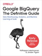
A Deep Neural Network (DNN) can be thought of as an extension of linear models in which each node in the first layer consists of a weighted sum of the input features transformed through a (typically nonlinear) function. The second layer consists of nodes, each of which is a weighted sum of the outputs of the first layer transformed through a nonlinear function, and so on, as demonstrated in Figure 9-5.
Figure 9-5. A Deep Neural Network consists of layers of “nodes.” This example shows two layers between the inputs and outputs and each layer with three nodes, but we can have an arbitrary number of layers and an arbitrary number of nodes in each layer.
To train a DNN model with 64 nodes in the first layer and 32 nodes in the second layer, you would do the following:
CREATE OR REPLACE MODEL ch09eu.bicycle_model_dnn
TRANSFORM(* EXCEPT(start_date)
           , IF(EXTRACT(dayofweek FROM start_date) BETWEEN 2 and 6, 'weekday',
'weekend') as dayofweek
           , ML.BUCKETIZE(EXTRACT(HOUR FROM start_date), [5, 10, 17]) AS hourofday
)
OPTIONS(input_label_cols=['duration'],
        model_type='dnn_regressor',
        hidden_units=[64, 32])
AS

SELECT
  duration
  , start_station_name
  , start_date
FROM `bigquery-public-data`.london_bicycles.cycle_hire
This model took about 20 minutes to train. It ended with a mean absolute error of 1,016 seconds. This is, of course, worse than the 901 seconds that we achieved with the linear model. Sadly, this is par for the course—DNNs are notoriously finicky to train.
Tip
We strongly recommend that you begin with linear models, and only after you have finalized the set of features and transformations should you move on to experiment with more complex models. This is because with the dnn_regressor you will probably need to experiment with different numbers of layers and nodes (i.e., with hidden_units) and regularization settings (i.e., with l2_reg) to obtain good performance. Considering how finicky deep learning networks can be to train, varying feature representations at the same time is a surefire recipe for confusion.
One way to handle this finickiness is to perform hyperparameter tuning to search for optimal network parameters—this is supported by a full-fledged machine learning framework like Cloud AI Platform (CAIP).10 You might be better off doing this training there, or using AutoML (we explore both of these options later in this chapter), but for now let’s try using a smaller network:
CREATE OR REPLACE MODEL ch09eu.bicycle_model_dnn
 TRANSFORM(* EXCEPT(start_date)
           , IF(EXTRACT(dayofweek FROM start_date) BETWEEN 2 and 6, 'weekday',
'weekend') as dayofweek
           , ML.BUCKETIZE(EXTRACT(HOUR FROM start_date), [5, 10, 17]) AS hourofday
)
OPTIONS(input_label_cols=['duration'],
        model_type='dnn_regressor',
         hidden_units=[10, 5])
AS

SELECT
  duration
  , start_station_name
  , start_date
FROM `bigquery-public-data`.london_bicycles.cycle_hire
This yields better performance (981 seconds) but is still not as good as the linear model. More hyperparameter tuning is needed to get a DNN model that does better than the linear model we started out with. Also, in general a DNN provides superior performance only if there are many continuous features.
Gradient-boosted trees
Decision trees are a popular technique in machine learning because of their ready interpretability (they are essentially just combinations of if-then rules). However, decision trees tend to have poor accuracy because the range of functions they can approximate is limited and can be prone to overfitting. One way of improving the performance of decision trees (at the expense of explainability11) is to train an ensemble of decision trees, each of which is a poor predictor but when averaged together yield good performance. Boosting is a technique that is used to select trees in the ensemble, and XGBoost12 is a scalable, distributed way to build boosted decision trees on extremely large and sparse datasets. XGBoost used to be considered the state-of-the-art machine learning technique until the advent of deep learning networks circa 2015. It continues to be popular on structured data problems.
You can train an XGBoost machine learning model in BigQuery by selecting the boosted_tree_regressor model type:
CREATE OR REPLACE MODEL ch09eu.bicycle_model_xgboost
TRANSFORM(* EXCEPT(start_date)
          , IF(EXTRACT(dayofweek FROM start_date) BETWEEN 2 and 6,
     'weekday', 'weekend') as dayofweek
          , ML.BUCKETIZE(EXTRACT(HOUR FROM start_date), [5, 10, 17]) AS hourofday
)
OPTIONS(input_label_cols=['duration'],
        model_type='boosted_tree_regressor',
        max_tree_depth=4)
AS

SELECT
  duration
  , start_station_name
  , start_date
FROM `bigquery-public-data`.london_bicycles.cycle_hire
The resulting model on this problem has poorer performance (1,363 seconds) than the linear model. The importance of the input features can be obtained by using this command:
SELECT * FROM ML.FEATURE_INFO(MODEL ch09eu.bicycle_model_xgboost)
Human insights and auxiliary data
Besides trying different model architectures and tuning the parameters of these models, we might consider adding new input features that incorporate human insights or provide auxiliary data to the machine learning model.
For example, in the previous model, we used ML.BUCKETIZE to split a continuous variable (the hour extracted from the timestamp) into four bins. Another extremely useful function is ML.FEATURE_CROSS, which can combine separate categorical features into an AND condition (this sort of relationship between features can be difficult for a machine learning model to learn). In our problem, intuition dictates that the combination of weekday and morning is a good predictor of bicycle rental duration, much more so than either weekday by itself or morning by itself. If so, it might be worthwhile to create a feature cross of the two features instead of treating the day and time separately:
ML.FEATURE_CROSS(STRUCT(
   IF(EXTRACT(dayofweek FROM start_date) BETWEEN 2 and 6,
       'weekday', 'weekend') as dayofweek,
   ML.BUCKETIZE(EXTRACT(HOUR FROM start_date),
       [5, 10, 17]) AS hr
)) AS dayhr
In our models so far, we used start_station_name as an input to the model. This treats the stations as independent. In Chapter 8, we discussed the benefits of ST_GeoHash as a way to capture spatial proximity. Let’s, therefore, bring in the auxiliary information about the stations’ locations and use that as an additional input to the model.
Combining these two ideas, we now have the model training query:
CREATE OR REPLACE MODEL ch09eu.bicycle_model_fc_geo
 TRANSFORM(duration
       , ML.FEATURE_CROSS(STRUCT(
           IF(EXTRACT(dayofweek FROM start_date) BETWEEN 2 and 6,
              'weekday', 'weekend') as dayofweek,
           ML.BUCKETIZE(EXTRACT(HOUR FROM start_date),
              [5, 10, 17]) AS hr
         )) AS dayhr
       , ST_GeoHash(ST_GeogPoint(latitude, longitude), 4) AS start_station_loc4
       , ST_GeoHash(ST_GeogPoint(latitude, longitude), 6) AS start_station_loc6
       , ST_GeoHash(ST_GeogPoint(latitude, longitude), 8) AS start_station_loc8
)
OPTIONS(input_label_cols=['duration'], model_type='linear_reg')
AS

SELECT
  duration
  , latitude
  , longitude
  , start_date
FROM `bigquery-public-data`.london_bicycles.cycle_hire
JOIN `bigquery-public-data`.london_bicycles.cycle_stations
ON cycle_hire.start_station_id = cycle_stations.id
This model results in a mean absolute error of 898 seconds, an improvement over the 901 seconds we saw earlier. However, the improvement is relatively minor. Because of these diminishing returns, it might be time to move on.
Building a Classification Model
In the previous section, we built machine learning models to predict the duration of a bicycle rental. However, over the span of one hour, many bicycles will be rented, and they will be rented for different durations. For example, take the distribution of bicycles that were rented at Royal Avenue 1, Chelsea, on weekdays in the hour starting at 14:00 (2:00 p.m.):
SELECT
  APPROX_QUANTILES(duration, 10) AS q
FROM `bigquery-public-data`.london_bicycles.cycle_hire
WHERE
  EXTRACT(dayofweek FROM start_date) BETWEEN 2 and 6
  AND EXTRACT(hour FROM start_date) = 14
  AND start_station_name = 'Royal Avenue 1, Chelsea'
Here’s the result:
| Row | q |
|---|---|
| 1 | 0 |
| 240 | |
| 420 | |
| 540 | |
| 660 | |
| 840 | |
| 1020 | |
| 1260 | |
| 1500 | |
| 2040 | |
| 386460 |
80% of weekday rentals at this station lasted less than 1,500 seconds. Had this been the only prediction for you to go by, you would have stocked only commuter bikes at this station on those days. However, had you known that somewhere between 10% and 20% of bicycle rentals last longer than 1,800 seconds, you might have decided to stock this station so that 15% of the bicycles are road bikes. A classification model will allow us to predict the probability that a rental will last longer than 1,800 seconds.
Training
For simplicity, let’s take the set of features we used in the regression model and train a model to predict the probability that the rental will be for longer than 30 minutes:
CREATE OR REPLACE MODEL ch09eu.bicycle_model_longrental
TRANSFORM(* EXCEPT(start_date)
          , IF(EXTRACT(dayofweek FROM start_date) BETWEEN 2 and 6,
     'weekday', 'weekend') as dayofweek
          , ML.BUCKETIZE(EXTRACT(HOUR FROM start_date), [5, 10, 17]) AS hourofday
)
OPTIONS(input_label_cols=['biketype'], model_type='logistic_reg')
AS

SELECT
  IF(duration > 1800, 'roadbike', 'commuter') AS biketype
  , start_station_name
  , start_date
FROM `bigquery-public-data`.london_bicycles.cycle_hire
Note that the model_type now is logistic regression (logistic_reg)—this is the simplest model type for classification problems. For classification with DNNs or boosted-regression trees, use dnn_classifier or boosted_tree_classifier, respectively.
We created the label by thresholding rentals at 1,800 seconds and gave the two categories the names roadbike and commuter (this is similar to how we created a categorical variable weekend/weekday from the numeric variable dayofweek). We could also have used a Boolean value (True/False), but using the actual category name is clearer.
At the end of training, you can see that the error has decreased over seven iterations through the dataset and has now converged, as depicted in Figure 9-6 (because of random seeds, your results might be somewhat different).
There are actually two loss curves in Figure 9-6: one on the training data and the other on the evaluation data (BigQuery automatically split the data for us). Here, the curves are quite similar. If the evaluation curve were much higher than the loss curve, you’d have been worried about overfitting. Switching to the table view, you can verify that the two losses were, indeed, quite similar throughout the training:
| Iteration | Training Data Loss | Evaluation Data Loss | Learn Rate | Duration (seconds) |
|---|---|---|---|---|
| 6 | 0.3072 | 0.3024 | 3.2000 | 41.59 |
| 5 | 0.3078 | 0.3029 | 6.4000 | 39.66 |
| 4 | 0.3119 | 0.3069 | 3.2000 | 40.54 |
| 3 | 0.3240 | 0.3195 | 1.6000 | 42.15 |
| 2 | 0.3576 | 0.3543 | 0.8000 | 37.96 |
| 1 | 0.4502 | 0.4483 | 0.4000 | 38.01 |
| 0 | 0.5812 | 0.5805 | 0.2000 | 22.10 |

Figure 9-6. The loss curve during model training has converged
Evaluation
The loss measure used in classification is cross-entropy, so that’s what the training curves depicted. You can look at more familiar evaluation metrics such as accuracy in the evaluation tab of the BigQuery web user interface (UI), as shown in Figure 9-7.

Figure 9-7. The evaluation tab in the BigQuery web UI for a classification model
Prediction
The prediction is similar to the regression case, except that you now get the probability of each class:
SELECT * FROM ML.PREDICT(MODEL ch09eu.bicycle_model_longrental,
  (SELECT 'Park Lane , Hyde Park' AS start_station_name
           , TIMESTAMP('2019-05-09 16:16:00 UTC') AS start_date)
)
This yields the following:
| Row | predicted_biketype | predicted_biketype_probs.label | predicted_biketype_probs.prob | start_station_name | start_date |
|---|---|---|---|---|---|
| 1 | commuter | roadbike | 0.4419... | Park Lane, Hyde Park | 2019-05-10 16:16:00 UTC |
| commuter | 0.5580... |
Thus, the probability that a rental at 4 p.m. on a weekday from Hyde Park will require a road bike is 0.44, or 44%. Ideally, then, you should have 44% of your bicycles at that station at that time be road bikes.
Choosing the Threshold
In our use case, the actual probability is what is of interest. Often, though, in classification problems, the desired output is the predicted class, not just the probability. Thus, the predicted output (see previous section) includes not only the probability but also the class with the highest probability. In a binary classification problem, this is the same as thresholding the probability at 0.5 and choosing the “positive” class if the probability is more than 0.5.
Recall is the percentage of actual true values (true positives / total positives) at a particular threshold point. If the recall is high, you’ll get almost all of the things you’re looking for. However, setting a threshold point with a high recall can be dangerous, because you might get a lot of false positives as well. If the threshold is 0, everything is chosen, so you get a perfect recall.
The other important metric is precision, which is the percentage of true positives over the whole dataset. In other words, it is a way of saying, “Given I’ve predicted this to be true, what is the probability that I’m right?” If you set the threshold to 0, you get the proportion of true data in the dataset. (In other words, you predict everything to be true, so if 10% of the values are true, your precision will be 10%. This isn’t a very good classifier.)
The aggregate metrics in the evaluation tab (e.g., accuracy=0.89) are calculated based on the 0.5 threshold.
If you wanted to ensure that you have a road bike in stock 50% of the times that one is required, you would want to have a recall of 0.5 because you’d need to capture half of the long rides. You can use the slider in the evaluation tab to change the threshold to 0.144, as shown in Figure 9-8, so that you obtain the desired recall metric. Note that this comes at the expense of precision; at this threshold, the model will give you a precision of 0.26—only 26% of the trips that we predict will require road bikes will actually be longer than 30 minutes.13

Figure 9-8. Change the probability threshold to obtain a desired recall or precision
For binary classification models, the desired threshold can be passed to ML.PREDICT:
SELECT * FROM ML.PREDICT(MODEL ch09eu.bicycle_model_longrental,
  (SELECT 'Park Lane , Hyde Park' AS start_station_name
           , TIMESTAMP('2019-05-09 16:16:00 UTC') AS start_date),
  STRUCT(0.144 AS threshold)
)
Here is the result:
| Row | predicted_biketype | predicted_biketype_probs.label | predicted_biketype_probs.prob | start_station_name | start_date |
|---|---|---|---|---|---|
| 1 | roadbike | roadbike | 0.4419... | Park Lane, Hyde Park | 2019-05-09 16:16:00 UTC |
Note that the predicted_biketype now is roadbike, even though the probability corresponding to roadbike is less than the default threshold of 0.5.
Customizing BigQuery ML
By default, BigQuery ML makes reasonable choices for learning rate,14 scaling input features,15 splitting the data,16 and so on. The OPTIONS setting when creating a model provides a number of fine-grained ways to control the model creation. In this section, we discuss a few of them.
Controlling Data Split
By default on moderately sized datasets, BigQuery randomly selects 20% of the data and keeps it aside for evaluation. The training is carried out on only 80% of the data we provide. For tiny datasets (those under 500 rows), all of the data is used for training, and for large datasets (those over 50,000 rows), only 10,000 rows are used for evaluation. We can control what data is used for evaluation by means of three parameters: data_split_method, data_split_eval_fraction, and data_split_col, as listed in Table 9-2.
| Scenario | data_split_method |
data_split_eval_fraction |
data_split_col |
|---|---|---|---|
| Default | auto_split |
0.2 | n/a |
| Train on all the data | no_split |
n/a | n/a |
| Keep aside a randomly selected 10% of data for evaluation | random |
0.1 | n/a |
| Specifically identify which rows are for evaluation | custom |
n/a | colnameRows with Boolean value of True/NULL for this column are kept aside for evaluation. |
| Keep last 10% of rows for evaluation | seq |
0.1 (default is 0.2) |
colnameRows are ordered ASC on this column. |
A better measure of how well the model will perform after it’s deployed is to train it on the first 80% (ordered by time) of bicycle rentals in the dataset and then test it on the remaining 20%.17 That is, rather than splitting randomly, you’d train on the older trips and test on the newer ones:
CREATE OR REPLACE MODEL ch09eu.bicycle_model_bucketized_seq
TRANSFORM(* EXCEPT(start_date)
           , IF(EXTRACT(dayofweek FROM start_date) BETWEEN 2 and 6, 'weekday',
'weekend') as dayofweek
           , ML.BUCKETIZE(EXTRACT(HOUR FROM start_date), [5, 10, 17]) AS hourofday
           , start_date—used to split the data
)
OPTIONS(input_label_cols=['duration'], model_type='linear_reg',
         data_split_method='seq',
         data_split_eval_fraction=0.2,
         data_split_col='start_date')
AS

SELECT
  duration
  , start_station_name
  , start_date
FROM `bigquery-public-data`.london_bicycles.cycle_hire
Note that the SELECT and TRANSFORM clauses both emit the column used to split the data, and that OPTIONS includes the three parameters that control how the data is split.
The mean absolute error now is 860 seconds, but we cannot compare this number with the results obtained with the random split—evaluation metrics depend quite heavily on what data is used for evaluation, and because we are using a different evaluation dataset now, we cannot compare these results to the ones obtained earlier. Also, our earlier results were contaminated by leakage—for example, of Christmas days.
Balancing Classes
In our classification problem, less than 12% of rentals last longer than 1,800 seconds. This is an example of an unbalanced dataset. It can be helpful to weight the rarer class higher, and we can do that either by passing in an explicit array of class weights or by asking BigQuery to set the weights of classes based on inverse frequency.
Here’s an example of using this autobalancing method:
CREATE OR REPLACE MODEL ch09eu.bicycle_model_longrental_balanced
TRANSFORM(* EXCEPT(start_date)
          , IF(EXTRACT(dayofweek FROM start_date) BETWEEN 2 and 6, 'weekday',
'weekend') as dayofweek
          , ML.BUCKETIZE(EXTRACT(HOUR FROM start_date), [5, 10, 17]) AS hourofday
          , start_date
)
OPTIONS(input_label_cols=['biketype'], model_type='logistic_reg',
        data_split_method='seq',
        data_split_eval_fraction=0.2,
        data_split_col='start_date',
        auto_class_weights=True)

AS

SELECT
  IF(duration > 1800, 'roadbike', 'commuter') AS biketype
  , start_station_name
  , start_date
FROM `bigquery-public-data`.london_bicycles.cycle_hire
Note that after you balance the weights, the probability that comes from the model is no longer an estimate of the actual predicted occurrence frequency. This is because the probability estimate that comes out of logistic regression is based on the frequency of occurrence in the data seen by the model, and we have artificially boosted the occurrence of rare events.
Regularization
Recall that in our data exploration, we discovered that except for a handful of stations which had unusually long durations, most of the stations had nearly identical durations, and many of these stations had very few rentals. Categorical features with such long-tailed distributions can cause overfitting. Overfitting is when the model learns noise (arbitrary variation) in the data, not the signal. In other words, the model can become so elaborate that it represents the dataset itself, not the underlying qualities of the dataset.
Regularization avoids overfitting because it penalizes complexity, in part by assigning penalties to large weight values. Large weight values are often a sign of overfitting because they can turn on suddenly when exactly one datapoint is encountered.
BigQuery ML supports two types of regularization: L1 and L2. L1 regularization tries to push individual weights to zero and is better for interpretability, whereas L2 tries to keep all the weights relatively similar and does better at controlling overfitting.18 You can control the amount of L1 or L2 regularization when creating the model:
CREATE OR REPLACE MODEL ch09eu.bicycle_model_bucketized_seq_l2
TRANSFORM(* EXCEPT(start_date)
          , IF(EXTRACT(dayofweek FROM start_date) BETWEEN 2 and 6,
                'weekday', 'weekend') as dayofweek
          , ML.BUCKETIZE(EXTRACT(HOUR FROM start_date), [5, 10, 17]) AS hourofday
          , start_date—used to split the data
)
OPTIONS(input_label_cols=['duration'], model_type='linear_reg',
         data_split_method='seq',
         data_split_eval_fraction=0.2,
         data_split_col='start_date',
         l2_reg=0.1)
AS

SELECT
  duration
  , start_station_name
  , start_date
FROM `bigquery-public-data`.london_bicycles.cycle_hire
In this case, though, the resulting mean absolute error is 857 seconds, nearly identical to what was obtained without L2 regularization; this is most likely because we have a large-enough dataset and a model with few enough parameters to tune that overfitting was not happening. L2 regularization is generally considered a best practice, particularly if you don’t have a large amount of data or if you are using a more sophisticated model (such as a DNN) with many more parameters.
k-Means Clustering
The machine learning algorithms that we have considered so far have been supervised learning methods—we needed to provide BigQuery a label column. BigQuery also supports unsupervised learning in that you can apply the k-means algorithm to group your data into clusters based on similarity. The algorithm is called k-means because it identifies k clusters, each of which is described in terms of the mean of the members of the cluster. Unlike supervised machine learning, which helps you predict the value of the label column when given values for the futures, unsupervised learning is descriptive. Use model_type=kmeans in BigQuery to understand your data in terms of centroids of the k clusters that have been determined from the data, and to make decisions about the members of each cluster based on the attributes of its centroid.
What’s Being Clustered?
The first step in using k-means clustering is to determine what is being clustered and why you are doing it. Because tables in BigQuery tend to be flattened and describe multiple aspects, it helps to be clear about what each member of the cluster represents.
Suppose that you have data in which each row represents a retail customer transaction. There are several ways in which you could do the clustering on this table, and which one you choose depends on what you want to do with the clusters:
-
You could find natural groups among your customers. This is called customer segmentation. Data we use to perform the customer segmentation would be attributes that describe the customer making the transaction—these might include things like which store they visited, what items they bought, how much they paid, and so on. The reason to cluster these customers is that you want to understand what these groups of customers are like (these are called personas) so that you can design items that appeal to members of one of those groups by understanding the “centroid customer” of each cluster.
-
You could find natural groups among the items purchased. These are called product groups. Data we use to perform the product groups would be attributes that describe the item(s) being purchased in the transaction—these might include things like who purchased them, when they were purchased, which store they were purchased at, and so forth. The reason to cluster these items is that you want to understand the characteristics of a product group so that you can learn how to reduce cannibalization or improve cross-selling.
In both of these cases, we are using clustering as a heuristic to help make decisions — it’s too difficult to design individualized products or understand product interactions, so you design for groups of customers or groups of items.
Note that for the specific use case of product recommendations (recommending products to customers or targeting customers for a product), it is better to train a matrix_factorization model as described later in this chapter. But for other decisions for which there is no readily available predictive analytics approach, k-means clustering might give you a way to make a data-driven decision.
Clustering Bicycle Stations
Suppose that you often make decisions about bicycle stations—which stations to stock with new types of bicycles, which ones to repair, which ones to expand, and so on, and you want to make these decisions in a data-driven manner. This means that you are going to cluster bicycle stations, and you could group stations that are similar based on attributes such as the duration of rentals from the station, the number of trips per day from the station, the number of bike racks at the station, and the distance of the station from the city center. Because the first two attributes vary based on whether the day in question is a weekday or a weekend, let’s compute two values for those.
Because the query is quite long and cumbersome, let’s also save it into a table:
CREATE OR REPLACE TABLE ch09eu.stationstats AS

WITH hires AS (
  SELECT
    h.start_station_name as station_name,
    IF(EXTRACT(DAYOFWEEK FROM h.start_date) BETWEEN 2 and 6,
               "weekday", "weekend") as isweekday,
    h.duration,
    s.bikes_count,
    ST_DISTANCE(ST_GEOGPOINT(s.longitude, s.latitude),
                ST_GEOGPOINT(-0.1, 51.5))/1000 as distance_from_city_center
  FROM `bigquery-public-data.london_bicycles.cycle_hire` as h
  JOIN `bigquery-public-data.london_bicycles.cycle_stations` as s
  ON h.start_station_id = s.id
  WHERE EXTRACT(YEAR from start_date) = 2015
),

stationstats AS (
  SELECT
     station_name,
     AVG(IF(isweekday = 'weekday', duration, NULL)) AS duration_weekdays,
     AVG(IF(isweekday = 'weekend', duration, NULL)) AS duration_weekends,
     COUNT(IF(isweekday = 'weekday', duration, NULL)) AS numtrips_weekdays,
     COUNT(IF(isweekday = 'weekend', duration, NULL)) AS numtrips_weekends,
     MAX(bikes_count) as bikes_count,
     MAX(distance_from_city_center) as distance_from_city_center
  FROM hires
  GROUP BY station_name
)

SELECT *
from stationstats
The resulting table has 802 rows, one for each station operating in 2015, and looks something like this:
| Row | station_name | duration_weekdays | duration_weekends | numtrips_weekdays | numtrips_weekends | bikes_count | distance_from_city_center |
|---|---|---|---|---|---|---|---|
| 1 | Borough Road, Elephant & Castle | 1109.932... | 2125.095... | 5749 | 1774 | 29 | 0.126... |
| 2 | Webber Street, Southwark | 795.439... | 938.357... | 6517 | 1619 | 34 | 0.164... |
| 3 | Great Suffolk Street, The Borough | 802.530... | 1018.310... | 8418 | 2024 | 18 | 0.193... |
Carrying Out Clustering
As with supervised learning, carrying out clustering simply involves a CREATE MODEL statement on the table created in the previous section, but taking care to remove the station_name field because it uniquely identifies each station:
CREATE OR REPLACE MODEL ch09eu.london_station_clusters
OPTIONS(model_type='kmeans',
        num_clusters=4,
        standardize_features = true) AS

SELECT * EXCEPT(station_name)
from ch09eu.stationstats
The model_type is kmeans. If the num_clusters option is omitted, BigQuery will choose a reasonable value based on the number of rows in the table. The other option, standardize_features, is necessary for this dataset because the different columns all have very different ranges. The distance from the city center is on the order of a few kilometers, whereas the number of trips and duration are on the order of thousands. Therefore, it is a good idea to have BigQuery scale these values by making them zero-mean and unit-variance.
Understanding the Clusters
To find which cluster a particular station belongs to, use ML.PREDICT. Here’s a query to find the cluster of every station that has “Kennington” in its name:
SELECT * except(nearest_centroids_distance)
FROM ML.PREDICT(MODEL ch09eu.london_station_clusters,
(SELECT * FROM ch09eu.stationstats
 WHERE REGEXP_CONTAINS(station_name, 'Kennington')))
This yields the following:
| Row | CENTROID_ID | station_name | duration_weekdays | duration_weekends | numtrips_weekdays | numtrips_weekends | bikes_count | distance_from_city_center |
|---|---|---|---|---|---|---|---|---|
| 1 | 2 | Kennington Road, Vauxhall | 1209.433... | 1720.598... | 8135 | 2975 | 26 | 0.891... |
| 2 | 2 | Kennington Lane Rail Bridge, Vauxhall | 979.391... | 1812.217... | 20263 | 5014 | 28 | 2.175... |
| 3 | 2 | Cotton Garden Estate, Kennington | 1572.919... | 997.949... | 5313 | 1600 | 14 | 1.117... |
| 4 | 3 | Kennington Station, Kennington | 1689.587... | 3579.285... | 4875 | 1848 | 15 | 1.298... |
A few of the Kennington stations are in centroid #2, whereas others are in centroid #3.19 To understand these groups, you can examine the centroid attributes:
SELECT *
FROM ML.CENTROIDS(MODEL ch09eu.london_station_clusters)
ORDER BY centroid_id
This returns a table that contains one row for each attribute of the cluster:
| Row | centroid_id | feature | numerical_value | categorical_value.category | categorical_value.value |
|---|---|---|---|---|---|
| 1 | 1 | distance_from_city_center | 2.978... | ||
| 2 | 1 | bikes_count | 10.013... | ||
| 3 | 1 | numtrips_weekends | 8273.849... |
You can pivot the table as follows:
CREATE TEMP FUNCTION cvalue(x ANY TYPE, col STRING) AS (
  (SELECT value from unnest(x) WHERE name = col)
);

WITH T AS (
  SELECT
  centroid_id,
  ARRAY_AGG(STRUCT(feature AS name,
                 ROUND(numerical_value,1) AS value)
          ORDER BY centroid_id) AS cluster
  FROM ML.CENTROIDS(MODEL ch09eu.london_station_clusters)
  GROUP BY centroid_id
)
SELECT
  CONCAT('Cluster#', CAST(centroid_id AS STRING)) AS centroid,
  cvalue(cluster, 'duration_weekdays') AS duration_weekdays,
  cvalue(cluster, 'duration_weekends') AS duration_weekends,
  cvalue(cluster, 'numtrips_weekdays') AS numtrips_weekdays,
  cvalue(cluster, 'numtrips_weekends') AS numtrips_weekends,
  cvalue(cluster, 'bikes_count') AS bikes_count,
  cvalue(cluster, 'distance_from_city_center') AS distance_from_city_center
FROM T
ORDER BY centroid_id ASC
The pivot gives you the following result:
| Row | centroid | duration_weekdays | duration_weekends | numtrips_weekdays | numtrips_weekends | bikes_count | distance_from_city_center |
|---|---|---|---|---|---|---|---|
| 1 | Cluster#1 | 1362.6 | 1968.4 | 25427.3 | 8273.8 | 10.0 | 3.0 |
| 2 | Cluster#2 | 1193.5 | 1738.1 | 8457.4 | 2584.3 | 21.0 | 3.0 |
| 3 | Cluster#3 | 1675.0 | 2460.5 | 4702.4 | 2136.8 | 14.9 | 6.7 |
| 4 | Cluster#4 | 1124.0 | 1543.1 | 8519.0 | 2342.1 | 5.7 | 4.1 |
To visualize this table, in the BigQuery web UI, click “Explore in Data Studio” and then select “Table with bars.” Make the centroid column the “dimension” and the remaining columns the metrics. Figure 9-9 shows the result.

Figure 9-9. Cluster attributes
From Figure 9-9, you can see that Cluster #1 consists of extremely busy stations (see the number of trips) that are close to the city center, Cluster #2 consists of less busy stations close to the city center, Cluster #3 consists of stations that are far away from the city center and seem to be used more on weekends on long trips (these are the only stations with more weekend trips than weekday trips), and Cluster #4 consists of tiny stations (see bikes_count) in the outer core of the city, probably in residential areas. Based on these characteristics and some knowledge of London, we can come up with descriptive names for these clusters. Cluster 1 would probably be “Tourist areas,” Cluster 2 would be “Business district,” Cluster 3 would be “Day trips,” and Cluster 4 would be “Commuter stations.”
Data-Driven Decisions
You can now use these clusters to make different decisions. For example, suppose that you just received funding and can expand the bike racks. In which stations should you install extra capacity? If you didn’t have the clustering data, you might be tempted to go with stations with lots of trips and not enough bikes — stations in Cluster #1. But you have done the clustering and discovered that this group of stations mostly serves tourists. They don’t vote, so let’s put the extra capacity in Cluster #4 (commuter stations).
To take another example, suppose that you need to experiment with a new type of lock. In which cluster of stations should you conduct this experiment? The business district stations seem logical, and sure enough, those are the stations with lots of bikes and that are busy enough to support an A/B test. If, on the other hand, you want to stock some stations with road (racing) bikes, which ones should you select? Cluster #3, comprising stations that serve people who are going on day trips out of the city, seems like a good choice.
Obviously, you could have made these decisions individually by doing custom data analysis each time. But clustering the stations, coming up with descriptive names, and using the names to make decisions is much simpler and more explainable.
Recommender Systems
Collaborative filtering provides a way to generate product recommendations for users, or user targeting for products. The starting point is a table with three columns: a user ID, an item ID, and the rating that the user gave the product. This table can be sparse—users don’t need to rate all products. Based on just the ratings, the technique finds similar users and similar products and determines the rating that a user would give an unseen product. Then we can recommend the products with the highest predicted ratings to users, or target products at users with the highest predicted ratings.
The MovieLens Dataset
To illustrate recommender systems in action, let’s use the MovieLens dataset. This is a dataset of movie reviews released by GroupLens, a research lab in the Department of Computer Science and Engineering at the University of Minnesota, through funding from the US National Science Foundation.
In Cloud Shell, download the data and load it as a BigQuery table using the following:
curl -O 'http://files.grouplens.org/datasets/movielens/ml-20m.zip'
unzip ml-20m.zip
bq --location=EU load --source_format=CSV
     --autodetect ch09eu.movielens_ratings ml-20m/ratings.csv
bq --location=EU load --source_format=CSV
     --autodetect ch09eu.movielens_movies_raw ml-20m/movies.csv
The resulting ratings table has the following columns:
| Row | userId | movieId | rating | timestamp | |
|---|---|---|---|---|---|
| 1 | 70141 | 6219 | 2.0 | 1070338674 | |
| 2 | 70159 | 2657 | 2.0 | 1427155558 |
Here’s a quick exploratory query:
SELECT
 COUNT(DISTINCT userId) numUsers,
 COUNT(DISTINCT movieId) numMovies,
 COUNT(*) totalRatings
FROM ch09eu.movielens_ratings
This reveals that the dataset consists of more than 138,000 users, nearly 27,000 movies, and a little more than 20 million ratings, confirming that the data has been loaded successfully.
Let’s examine the first few movies using the following query:
SELECT *
FROM ch09eu.movielens_movies_raw
WHERE movieId < 5
We can see that the genres column is a formatted string:
| Row | movieId | title | genres |
|---|---|---|---|
| 1 | 3 | Grumpier Old Men (1995) | Comedy|Romance |
| 2 | 4 | Waiting to Exhale (1995) | Comedy|Drama|Romance |
| 3 | 2 | Jumanji (1995) | Adventure|Children|Fantasy |
We can parse the genres into an array and rewrite the table as follows:
CREATE OR REPLACE TABLE ch09eu.movielens_movies AS
SELECT
* REPLACE(SPLIT(genres, "|") AS genres)
FROM
ch09eu.movielens_movies_raw
Now the table looks as follows:
| Row | movieId | title | genres |
|---|---|---|---|
| 1 | 4 | Waiting to Exhale (1995) | Comedy |
| Drama | |||
| Romance | |||
| 2 | 3 | Grumpier Old Men (1995) | Comedy |
| Romance | |||
| 3 | 2 | Jumanji (1995) | Adventure |
| Children | |||
| Fantasy |
With the MovieLens data now loaded, we are ready to do collaborative filtering.
Matrix Factorization
Matrix factorization is a collaborative filtering technique that relies on factorizing the ratings matrix into two vectors called the user factors and the item factors. The user factors vector is a low-dimensional representation of a user_col, and the item factors vector similarly represents an item_col.
You can create the recommender model using the following:
-- not the final model; see movie_recommender_16
CREATE OR REPLACE MODEL ch09eu.movie_recommender
options(model_type='matrix_factorization',
        user_col='userId', item_col='movieId', rating_col='rating')
AS

SELECT
userId, movieId, rating
FROM ch09eu.movielens_ratings
Note that you create a model as usual, except that the model_type is matrix_factorization and that you need to identify which columns play what roles in the collaborative filtering setup.
The resulting model took an hour to train, and the training data loss starts out extremely bad and is driven down to near-zero over the next four iterations:20
| Iteration | Training Data Loss | Evaluation Data Loss | Duration (seconds) | |
|---|---|---|---|---|
| 4 | 0.5734 | 172.4057 | 180.99 | |
| 3 | 0.5826 | 187.2103 | 1,040.06 | |
| 2 | 0.6531 | 4,758.2944 | 219.46 | |
| 1 | 1.9776 | 6,297.2573 | 1,093.76 | |
| 0 | 63,287,833,220.5795 | 168,995,333.0464 | 1,091.21 |
However, the evaluation data loss is quite high—much higher than the training data loss. This indicates that overfitting is happening, and so you need to add some regularization. Let’s do that next:
-- not final model. See movie_recommender_16
CREATE OR REPLACE MODEL ch09eu.movie_recommender_l2
options(model_type='matrix_factorization',
        user_col='userId', item_col='movieId',
        rating_col='rating', l2_reg=0.2)
AS

SELECT
userId, movieId, rating
FROM ch09eu.movielens_ratings
Now you get faster convergence (three iterations instead of five) and a lot less overfitting:
| Iteration | Training Data Loss | Evaluation Data Loss | Duration (seconds) | |
|---|---|---|---|---|
| 2 | 0.6509 | 1.4596 | 198.17 | |
| 1 | 1.9829 | 33,814.3017 | 1,066.06 | |
| 0 | 481,434,346,060.7928 | 2,156,993,687.7928 | 1,024.59 |
By default, BigQuery sets the number of factors to be the log2 of the number of rows. In this case, because we have 20 million rows in the table, the number of factors would have been chosen to be 24. As with the number of clusters in k-means clustering, this is a reasonable default, but it is often worth experimenting with a number about 50% higher (36) and a number that is about a third lower (16):21
CREATE OR REPLACE MODEL ch09eu.movie_recommender_16
options(model_type='matrix_factorization',
        user_col='userId', item_col='movieId',
        rating_col='rating', l2_reg=0.2, num_factors=16)
AS

SELECT
userId, movieId, rating
FROM ch09eu.movielens_ratings
When we did that, we discovered that the evaluation loss was lower (0.97) with num_factors=16 than with num_factors=36 (1.67) or num_factors=24 (1.45). We could continue experimenting, but we are likely to see diminishing returns with further experimentation. So let’s pick this as the final matrix factorization model and move on.
Making Recommendations
With the trained model, you can now provide recommendations. For example, let’s find the best comedy movies to recommend to the user whose userId is 903:
SELECT * FROM
ML.PREDICT(MODEL ch09eu.movie_recommender_16, (
  SELECT
     movieId, title, 903 AS userId
  FROM ch09eu.movielens_movies, UNNEST(genres) g
  WHERE g = 'Comedy'
))
ORDER BY predicted_rating DESC
LIMIT 5
In this query, we are calling ML.PREDICT, passing in the trained recommendation model and providing a set of movieId and userId on which to carry out the predictions. In this case, it’s just one userId (903), but all movies whose genre includes Comedy. Here is the result:
| Row | predicted_rating | movieId | title | userId |
|---|---|---|---|---|
| 1 | 4.747231361947591 | 107434 | Diplomatic Immunity (2009– ) | 903 |
| 2 | 4.372639637398302 | 62206 | Supermarket Woman (Sûpâ no onna) (1996) | 903 |
| 3 | 4.325021974040314 | 122441 | Tales That Witness Madness (1973) | 903 |
| 4 | 4.296062517241643 | 120313 | Otakus in Love (2004) | 903 |
| 5 | 4.277251207896746 | 130347 | Bill Hicks: Sane Man (1989) | 903 |
Filtering out previously rated movies
Of course, this includes movies the user has already seen and rated in the past. Let’s remove them:
SELECT * FROM
ML.PREDICT(MODEL ch09eu.movie_recommender_16, (
  WITH seen AS (
     SELECT ARRAY_AGG(movieId) AS movies
     FROM ch09eu.movielens_ratings
     WHERE userId = 903
  )
  SELECT
     movieId, title, 903 AS userId
  FROM ch09eu.movielens_movies, UNNEST(genres) g, seen
  WHERE g = 'Comedy' AND movieId NOT IN UNNEST(seen.movies)
))
ORDER BY predicted_rating DESC
LIMIT 5
For this user, this happens to yield the same set of movies—the top predicted ratings didn’t include any of the movies the user has already seen.
Customer targeting
In the previous section, we looked at how to identify the top-rated movies for a specific user. Sometimes we have a product and need to find the customers who are likely to appreciate it. Suppose, for example, you want to get more reviews for movieId=96481, which has only one rating, and you want to send coupons to the 100 users who are likely to rate it the highest. We can identify those users by using the following:
SELECT * FROM
ML.PREDICT(MODEL ch09eu.movie_recommender_16, (
  WITH allUsers AS (
      SELECT DISTINCT userId
      FROM ch09eu.movielens_ratings
  )
  SELECT
     96481 AS movieId,
     (SELECT title FROM ch09eu.movielens_movies WHERE movieId=96481) title,
     userId
  FROM
     allUsers
))
ORDER BY predicted_rating DESC
LIMIT 100
The result gives us 100 users to target, the top 5 of whom we list here:
| Row | predicted_rating | movieId | title | userId |
|---|---|---|---|---|
| 1 | 4.8586009640376915 | 96481 | American Mullet (2001) | 54192 |
| 2 | 4.670093338552966 | 96481 | American Mullet (2001) | 84240 |
| 3 | 4.544395037073204 | 96481 | American Mullet (2001) | 109638 |
| 4 | 4.422718574118088 | 96481 | American Mullet (2001) | 26606 |
| 5 | 4.410969328468145 | 96481 | American Mullet (2001) | 138139 |
Batch predictions for all users and movies
What if you want to carry out predictions for every user and movie combination? Instead of having to pull distinct users and movies as in the previous query, a convenient function is provided to carry out batch predictions for all movieId and userId encountered during training:
SELECT *
FROM ML.RECOMMEND(MODEL ch09eu.movie_recommender_16)
As seen in an earlier section, it is possible to filter out movies that the user has already seen and rated in the past. The reason previously viewed movies aren’t filtered out by default is that there are situations (think of restaurant recommendations, for example) for which it is perfectly expected that we would need to recommend restaurants the user has liked in the past.
Incorporating User and Movie Information
The matrix factorization approach does not use any information about users or movies beyond what is available from the ratings matrix. However, we will often have user information (such as the city they live in, their annual income, their annual expenditure, etc.), and we will almost always have more information about the products in our catalog. How do we incorporate this information into our recommendation model?
The answer lies in recognizing that the user factors and product factors that result from the matrix factorization approach end up being a concise representation of the information about users and products available from the ratings matrix. We can concatenate this information with other information we have available and train a regression model to predict the rating.
Obtaining user and product factors
You can get the user factors or product factors from ML.WEIGHTS. For example, here’s how to get the product factors for movieId=96481 and user factors for userId=54192:
SELECT
   processed_input
   , feature
   , TO_JSON_STRING(factor_weights)
   , intercept
FROM ML.WEIGHTS(MODEL ch09eu.movie_recommender_16)
WHERE
(processed_input = 'movieId' AND feature = '96481')
OR
(processed_input = 'userId' AND feature = '54192')
The result is as follows:
| Row | processed_input | feature | f0_ | intercept |
|---|---|---|---|---|
| 1 | movieId | 96481 | [{"factor”:16,"weight”:0.01274324364248563},{"factor”:15,"weight”:-0.026002830400362179},{"factor”:14,"weight”:-0.0088894978851240675},{"factor”:13,"weight”:0.010309411637259363},{"factor”:12,"weight”:-0.025990228913849212},{"factor”:11,"weight”:0.0037023423385396021},{"factor”:10,"weight”:-0.0016743710047063861},{"factor”:9,"weight”:0.018434530705228803},{"factor”:8,"weight”:-0.0016500835388799462},{"factor”:7,"weight”:-0.021652088589080184},{"factor”:6,"weight”:-0.00097969747732716637},{"factor”:5,"weight”:-0.056352201014532581},{"factor”:4,"weight”:-0.025090456181039382},{"factor”:3,"weight”:0.015317626028966519},{"factor”:2,"weight”:-0.00046084151232374118},{"factor”:1,"weight”:-0.0009461271544545048}] | -1.1915305828542884 |
| 2 | userId | 54192 | [{"factor”:16,"weight”:-0.66257902781387934},{"factor”:15,"weight”:-0.089502881890795027},{"factor”:14,"weight”:-0.14498342867805328},{"factor”:13,"weight”:0.57708118940369757},{"factor”:12,"weight”:-0.25409266698347688},{"factor”:11,"weight”:0.243523510689305},{"factor”:10,"weight”:0.48314159427498959},{"factor”:9,"weight”:0.21335694312220596},{"factor”:8,"weight”:0.34206958377350211},{"factor”:7,"weight”:-0.076313491055098021},{"factor”:6,"weight”:0.21214183741037482},{"factor”:5,"weight”:0.19387028511697624},{"factor”:4,"weight”:-0.42699681695332414},{"factor”:3,"weight”:0.046570444717220438},{"factor”:2,"weight”:0.25934273163373722},{"factor”:1,"weight”:-0.18839802656522864}] | 2.511409230366029 |
Multiplying these weights and adding the intercept is how you get the predicted rating for this combination of movieId and userId in the matrix factorization approach.
These weights also serve as a low-dimensional representation of the movie and user behavior. You can create a regression model to predict the rating given the user factors, product factors, and any other information that we know about our users and products.
Creating input features
The MovieLens dataset does not have any user information and has very little information about the movies themselves. To illustrate the concept, therefore, let’s create some synthetic information about users:
CREATE OR REPLACE TABLE ch09eu.movielens_users AS
SELECT
  userId
  , RAND() * COUNT(rating) AS loyalty
  , CONCAT(SUBSTR(CAST(userId AS STRING), 0, 2)) AS postcode
FROM
  ch09eu.movielens_ratings
GROUP BY userId
Input features about users can be obtained by joining the user table with the machine learning weights and selecting all of the user information and the user factors from the weights array:
WITH userFeatures AS (
  SELECT
      u.*,
      (SELECT ARRAY_AGG(weight) FROM UNNEST(factor_weights)) AS user_factors
  FROM
      ch09eu.movielens_users u
  JOIN
      ML.WEIGHTS(MODEL ch09eu.movie_recommender_16) w
   ON
      processed_input = 'userId' AND feature = CAST(u.userId AS STRING)
)

SELECT * FROM userFeatures
LIMIT 5
This yields user features like these (you will need to remove the userId itself before feeding it into the regression model):
| Row | userId | loyalty | postcode | user_factors |
|---|---|---|---|---|
| 1 | 65536 | 72.51794801197904 | 65 | 0.038901538776462 |
| 0.0019075355240976716 | ||||
| 0.011537776936285278 | ||||
| -0.0322503841197857 | ||||
| 0.046464397209825425 | ||||
| -0.015348467879503527 | ||||
| 0.05865111283285229 | ||||
| 0.04859058815259179 | ||||
| 0.017664456774125117 | ||||
| 0.006847553039523945 | ||||
| 0.012585216564478762 | ||||
| -0.06506297976701378 | ||||
| -0.005041156227839918 | ||||
| -0.04187860699038322 | ||||
| 0.006216526560890197 | ||||
| 0.02711744261644579 |
Similarly, you can get product features for the movies data, except that you need to decide how to handle the genre because a movie could have more than one. If you decide to create a separate training row for each genre, you can construct the product features using the following:
WITH productFeatures AS (
  SELECT
      p.* EXCEPT(genres)
      , g
      , (SELECT ARRAY_AGG(weight) FROM UNNEST(factor_weights)) AS product_factors
  FROM
      ch09eu.movielens_movies p, UNNEST(genres) g
  JOIN
      ML.WEIGHTS(MODEL ch09eu.movie_recommender_16) w
  ON
      processed_input = 'movieId' AND feature = CAST(p.movieId AS STRING)
)

SELECT * FROM productFeatures
LIMIT 5
This yields rows of the following form:
| Row | movieId | title | g | product_factors |
|---|---|---|---|---|
| 1 | 1450 | Prisoner of the Mountains (Kavkazsky plennik) (1996) | War | 0.9883690055578206 |
| 1.3052751077485096 | ||||
| -1.4000285383517228 | ||||
| 1.3901032474256991 | ||||
| -0.32863748198986686 | ||||
| -0.7688057246956399 | ||||
| -1.1853591273232054 | ||||
| -0.4553668299329251 | ||||
| -0.14564591302024543 | ||||
| -0.18609388556738163 | ||||
| -0.3547198526732644 | ||||
| 0.06067380147330148 | ||||
| -0.2733324088164271 | ||||
| 1.8302213060412562 | ||||
| 0.4753820155626278 | ||||
| 1.559946725190114 |
By combining these two WITH clauses and pulling in the rating corresponding to the movieId-userId combination (if it exists in the ratings table), you can create the training dataset:22
CREATE OR REPLACE TABLE ch09eu.movielens_hybrid_dataset AS

WITH userFeatures AS (
  SELECT
      u.*,
      (SELECT ARRAY_AGG(weight) FROM UNNEST(factor_weights)) AS user_factors
  FROM
      ch09eu.movielens_users u
  JOIN
      ML.WEIGHTS(MODEL ch09eu.movie_recommender_16) w
  ON
      processed_input = 'userId' AND feature = CAST(u.userId AS STRING)
),

productFeatures AS (
  SELECT
      p.* EXCEPT(genres)
      , g
      , (SELECT ARRAY_AGG(weight) FROM UNNEST(factor_weights)) AS product_factors
  FROM
      ch09eu.movielens_movies p, UNNEST(genres) g
  JOIN
      ML.WEIGHTS(MODEL ch09eu.movie_recommender_16) w
  ON
      processed_input = 'movieId' AND feature = CAST(p.movieId AS STRING)
)

SELECT p.* EXCEPT(movieId), u.* EXCEPT(userId), rating
FROM productFeatures p, userFeatures u
JOIN
   ch09eu.movielens_ratings r
ON
   r.movieId = p.movieId AND r.userId = u.userId
One of the rows of this table looks like this:
| 1 | Hunted, The (2003) | Action | 2.6029616190628015 | 692.7156232519949 | 70 | 0.026523240535672774 | 2.0 |
|---|---|---|---|---|---|---|---|
| 0.33485455845698525 | 0.0019319939217823622 | ||||||
| 0.31628840722516194 | -0.0020145595411925534 | ||||||
| -0.3075233831543138 | -0.002646563034985453 | ||||||
| -0.4473419662482839 | -0.01594551937825673 | ||||||
| -1.0222758233057185 | -0.010801066706191506 | ||||||
| -0.42418301494313826 | 4.772572135005211E-4 | ||||||
| -1.2447809221572947 | 0.014766024570817101 | ||||||
| -0.20242685993451942 | -0.007500869241538576 | ||||||
| 1.330350771422776 | -0.020383420117709883 | ||||||
| -0.3354935275410769 | -0.007863867111381763 | ||||||
| 0.32404375319192513 | 0.019901597021923123 | ||||||
| 1.402657314320568 | -0.003178194776711233 | ||||||
| 0.4728896971092763 | 0.013146874239054253 | ||||||
| -0.5743444547904143 | -0.0017117741950437 | ||||||
| 0.35632448579921905 | -0.030130776462043048 |
Essentially, you have a couple of attributes about the movie, the product factors array corresponding to the movie, a couple of attributes about the user, and the user factors array corresponding to the user. These form the inputs to the “hybrid” recommendations model that builds off the matrix factorization model and adds in metadata about users and movies.
Training hybrid recommendation model
As of this writing, BigQuery ML cannot handle arrays as inputs to a regression model. Let’s therefore define a function to convert arrays to a struct for which the array elements are its fields:
CREATE OR REPLACE FUNCTION ch09eu.arr_to_input_3(a ARRAY<FLOAT64>)
RETURNS STRUCT<a1 FLOAT64, a2 FLOAT64, a3 FLOAT64> AS (
STRUCT(
    a[OFFSET(0)]
    , a[OFFSET(1)]
    , a[OFFSET(2)]
));
Now you can do the following:
SELECT
  ch09eu.arr_to_input_3(a).*
FROM
(SELECT [34.23, 43.21, 63.21] AS a)
And here’s your result:
| Row | a1 | a2 | a3 |
|---|---|---|---|
| 1 | 34.23 | 43.21 | 63.21 |
You can create a similar function named ch09eu.arr_to_input_16_users to convert the user factor array into named columns, and a similar function for the product factor arrays.23 Then you can tie together metadata about users and products with the user factors and product factors obtained from the matrix factorization approach to create a regression model to predict the rating:
CREATE OR REPLACE MODEL ch09eu.movielens_recommender_hybrid
OPTIONS(model_type='linear_reg', input_label_cols=['rating'])
AS

SELECT
  * EXCEPT(user_factors, product_factors)
  , ch09eu.arr_to_input_16_users(user_factors).*
  , ch09eu.arr_to_input_16_products(product_factors).*
FROM
  ch09eu.movielens_hybrid_dataset
There is no point in looking at the evaluation metrics of this model, because the user information we used to create the training dataset was fake (note the RAND() in the creation of the loyalty column)—we did this exercise to demonstrate how it could be done. And of course, we could train a dnn_regressor model and optimize the hyperparameters if we want a more sophisticated model. But if we are going to go that far, it might be better to consider using AutoML tables, which we cover in the next section.
Custom Machine Learning Models on GCP
Whereas BigQuery ML provides you a choice of models24 that can be built and iterated over very quickly, AutoML provides you with a state-of-the-art, high-quality model for the task, with the trade-off being that the model takes hours or even days to train. Keras and TensorFlow provide lower-level control of machine learning model architectures and allow you to design, develop, and deploy custom machine learning models. We recommend that you begin with BigQuery ML for machine learning on structured or semi-structured data and, depending on your skill set and the value of the problem being solved, use AutoML or Keras to fine-tune the machine learning problem.
Hyperparameter Tuning
When you’re carrying out machine learning, there are many parameters that you choose rather arbitrarily. These include factors such as the learning rate, the level of L2 regularization, the number of layers and nodes in a neural network, the maximum depth of a boosted tree, and the number of factors of a matrix factorization model. It is often the case that choosing a different value for these could result in a better model (as measured by the error on a withheld evaluation dataset). Choosing a good value for these parameters is called hyperparameter tuning.
Hyperparameter tuning using scripting
Take the k-means clustering model. The evaluation tab in the BigQuery web UI (as well as SELECT * from ML.EVALUATE) shows the Davies-Bouldin index, which is useful for determining the optimal number of clusters supported by the data (the lower the number, the better the clustering).
For example, here’s a script to try varying the number of clusters:
DECLARE NUM_CLUSTERS INT64 DEFAULT 3;
DECLARE MIN_ERROR FLOAT64 DEFAULT 1000.0;
DECLARE BEST_NUM_CLUSTERS INT64 DEFAULT -1;
DECLARE MODEL_NAME STRING;

WHILE NUM_CLUSTERS < 8 DO

  SET MODEL_NAME = CONCAT('ch09eu.london_station_clusters_',
                          CAST(NUM_CLUSTERS AS STRING));

  CREATE OR REPLACE MODEL MODEL_NAME
  OPTIONS(model_type='kmeans',
           num_clusters=NUM_CLUSTERS,
           standardize_features = true) AS
  SELECT * except(station_name)
  from ch09eu.stationstats;

  SET error = (SELECT davies_bouldin_index FROM ML.EVALUATE(MODEL MODEL_NAME));
  IF error < MIN_ERROR THEN
      SET MIN_ERROR = error;
      SET BEST_NUM_CLUSTERS = NUM_CLUSTERS;
  END IF;


  SET NUM_CLUSTERS = NUM_CLUSTERS + 1;

END WHILE
Hyperparameter tuning in Python
Alternatively, you could do this using Python and its multithreading capability to limit the number of concurrent queries:25
def train_and_evaluate(num_clusters: Range, max_concurrent=3):
    # grid search means to try all possible values in range
    params = []
    for k in num_clusters.values():
        params.append(Params(k))

    # run all the jobs
    print('Grid search of {} possible parameters'.format(len(params)))
    pool = ThreadPool(max_concurrent)
    results = pool.map(lambda p: p.run(), params)

    # sort in ascending order
    return sorted(results, key=lambda p: p._error)
In this code, the run() method of the Params class invokes the appropriate training and evaluation queries:
class Params:
    def __init__(self, num_clusters):
        self._num_clusters = num_clusters
        self._model_name = (
            'ch09eu.london_station_clusters_{}'.format(num_clusters))
        self._train_query = """
          CREATE OR REPLACE MODEL {}
          OPTIONS(model_type='kmeans',
                  num_clusters={},
                  standardize_features = true) AS
          SELECT * except(station_name)
          from ch09eu.stationstats
        """.format(self._model_name, self._num_clusters)
        self._eval_query = """
          SELECT davies_bouldin_index AS error
          FROM ML.EVALUATE(MODEL {});
        """.format(self._model_name)
       self._error = None

    def run(self):
        bq = bigquery.Client(project=PROJECT)
        job = bq.query(self._train_query, location='EU')
        job.result() # wait for job to finish
        evaldf = bq.query(self._eval_query, location='EU').to_dataframe()
        self._error = evaldf['error'][0]
        return self
When searching in the range [3,9], you find that the number of clusters at which the error is minimized is 7:
ch09eu.london_station_clusters_7           1.551265     7
ch09eu.london_station_clusters_9           1.571020     9
ch09eu.london_station_clusters_6           1.571398     6
ch09eu.london_station_clusters_4           1.596398     4
ch09eu.london_station_clusters_8           1.621974     8
ch09eu.london_station_clusters_5           1.660766     5
ch09eu.london_station_clusters_3           1.681441     3
Hyperparameter tuning using AI Platform
In both of the hyperparameter tuning methods that we’ve considered so far, we tried out every possible value of a parameter that fell within a range. As the number of possible parameters grows, a grid search becomes increasingly wasteful. It is better to use a more efficient search algorithm, and that’s where Cloud AI Platform’s hyperparameter tuning can be helpful. You can use the hyperparameter tuning service for any model (not just TensorFlow). Let’s apply it to tuning the feature engineering and number of nodes of a DNN model.26
First, create a configuration file that specifies the ranges for each of the parameters, the number of concurrent queries, and the total number of trials:
trainingInput:
  scaleTier: CUSTOM
  masterType: standard   # See: https://cloud.google.com/ml-
engine/docs/tensorflow/machine-types
  hyperparameters:
     goal: MINIMIZE
     maxTrials: 50
     maxParallelTrials: 2
     hyperparameterMetricTag: mean_absolute_error
     params:
     - parameterName: afternoon_start
       type: INTEGER
       minValue: 9
       maxValue: 12
       scaleType: UNIT_LINEAR_SCALE
     - parameterName: afternoon_end
       type: INTEGER
       minValue: 15
       maxValue: 19
       scaleType: UNIT_LINEAR_SCALE
     - parameterName: num_nodes_0
       type: INTEGER
       minValue: 10
       maxValue: 100
       scaleType: UNIT_LOG_SCALE
     - parameterName: num_nodes_1
       type: INTEGER
       minValue: 3
       maxValue: 10
       scaleType: UNIT_LINEAR_SCALE
Note that we have specified minimum and maximum values for each of the parameters and the metric (mean absolute error) to be minimized. We are asking for optimization to happen using just 50 trials, whereas a grid search would have required trying out 4×4×90×7, or more than 10,000 options. So using the AI Platform hyperparameter tuning service results in a 200-fold savings!
Next, you create a Python program that invokes BigQuery to train and evaluate the model given a single set of these parameters:
def train_and_evaluate(args):
    model_name = "ch09eu.bicycle_model_dnn_{}_{}_{}_{}".format(
        args.afternoon_start, args.afternoon_end, args.num_nodes_0,
args.num_nodes_1
    )
    train_query = """
         CREATE OR REPLACE MODEL {}
         TRANSFORM(* EXCEPT(start_date)
                   , IF(EXTRACT(dayofweek FROM start_date) BETWEEN 2 and 6,
'weekday', 'weekend') as dayofweek
                   , ML.BUCKETIZE(EXTRACT(HOUR FROM start_date), [5, {}, {}]) AS
hourofday
         )
         OPTIONS(input_label_cols=['duration'],
                 model_type='dnn_regressor',
                 hidden_units=[{}, {}])
         AS

         SELECT
           duration
           , start_station_name
           , start_date
         FROM `bigquery-public-data`.london_bicycles.cycle_hire
     """.format(model_name,
                args.afternoon_start,
                args.afternoon_end,
                args.num_nodes_0,
                args.num_nodes_1)
     logging.info(train_query)
     bq = bigquery.Client(project=args.project,
                          location=args.location,
                          credentials=get_credentials())
     job = bq.query(train_query)
     job.result() # wait for job to finish

     eval_query = """
         SELECT mean_absolute_error
         FROM ML.EVALUATE(MODEL {})
     """.format(model_name)
     logging.info(eval_info)
     evaldf = bq.query(eval_query).to_dataframe()
     return evaldf['mean_absolute_error'][0]
Note that this code uses a specific value for each of the tunable parameters and returns the mean absolute error, which is the metric being minimized.
This error value is then written out:
hpt.report_hyperparameter_tuning_metric(
       hyperparameter_metric_tag='mean_absolute_error',
       metric_value=error,
       global_step=1)
The training program is submitted to the AI Platform Training service:
gcloud ai-platform jobs submit training $JOBNAME
  --runtime-version=1.13
  --python-version=3.5
  --region=$REGION
  --module-name=trainer.train_and_eval
  --package-path=$(pwd)/trainer
  --job-dir=gs://$BUCKET/hparam/
  --config=hyperparam.yaml
  —
  --project=$PROJECT --location=EU
The resulting output, shown in the AI Platform console, contains the best parameters.
AutoML
AutoML consists of a family of products that provide a code-free way to automatically create and deploy state-of-the-art machine learning models. They tend to rely on applying a variety of feature engineering, hyperparameter tuning, neural architecture search, transfer learning, and ensembling methods to build models that have comparable quality to models manually crafted by top machine learning experts.
Tip
Use BigQuery ML to formulate your machine learning problems—to identify the features and labels, to quickly diagnose whether some new dataset improves accuracy, to detect mistakes in assumptions about time-dependence, and to determine the best way of representing some piece of domain knowledge. The fast iteration capability that BigQuery ML provides is invaluable, as is the ability to train models without moving data outside the data warehouse. After you have identified a feasible machine learning problem, you can use AutoML to get a very accurate model on the specific training dataset (features and labels). In our experience, AutoML infused with features that represent the insights of domain experts is hard to beat either in terms of accuracy or in terms of time to deployment.
AutoML Vision, for example, provides a web-based interface to upload images (or point to images on Google Cloud Storage), identify their labels, and launch the training of image classification or object detection models.
Because the data in BigQuery tends to be structured or semi-structured, the AutoML models that are relevant tend to be AutoML Natural Language (to do tasks such as text classification and entity detection), AutoML Tables (to do tasks such as regression, classification, and time-series forecasting on structured data), and AutoML Recommendations (to build state-of-the-art recommendation models).
To use AutoML Tables (Figure 9-10), simply visit the starting point on the GCP console, point it at a BigQuery table, select the feature columns and label column, and then click Train. Although training will take much longer (on the order of 12 to 24 hours), the resulting accuracy tends to be higher than what you might have achieved on the same dataset with BigQuery ML.

Figure 9-10. AutoML Tables can start from a BigQuery table, the same training dataset that was built through iterative exploration and experimentation in BigQuery ML. In our experience, AutoML Tables applied to thoughtfully created training datasets provides state-of-the-art performance.
Support for TensorFlow
Even though BigQuery ML is scalable and convenient, and AutoML powerful and accurate, there are times when you might want to build your own custom models using Keras or TensorFlow. You might also find it advantageous to train models using TensorFlow and predict using BigQuery, or to train models in BigQuery but deploy into TensorFlow Serving.
It is possible to access BigQuery directly from TensorFlow code and to export BigQuery tables to TensorFlow records, transforming the data along the way. There is also interoperability between BigQuery and TensorFlow models—it is possible to load a TensorFlow model into BigQuery and to export a BigQuery model in TensorFlow’s SavedModel format. We cover these capabilities in this section.
TensorFlow’s BigQueryReader
A TensorFlow input pipeline can read from a BigQuery table into keyed TensorFlow Examples using BigQueryReader. First, create a features dictionary of the columns of interest:
features = dict(
  start_station_name=tf.FixedLenFeature([1], tf.string),
  duration=tf.FixedLenFeature([1], tf.int32))
Then create a reader specifying the timestamp at which the data is to be read (because the BigQuery table could be receiving streamed data while we are reading it) and the number of threads (partitions) in which the table is to be read:
reader = tf.contrib.cloud.BigQueryReader(project_id=PROJECT,
            dataset_id=DATASET,
            table_id=TABLE,
            timestamp_millis=TIME,
            num_partitions=NUM_PARTITIONS,
            features=features)
Finally, populate a queue with the BigQuery Table partitions, and use it to read the TensorFlow examples:
queue = tf.train.string_input_producer(reader.partitions())
row_id, examples_serialized = reader.read(queue)
examples = tf.parse_example(examples_serialized, features=features)
Although this works, there are several problems with this approach. In machine learning training, you will need to read batch_size records at once, shuffle the read order across workers, prefetch records, and so on. Hence, we recommend that you do not follow this approach.
Using pandas
If the BigQuery table is small enough, read it directly into an in-memory pandas DataFrame:
query = """
SELECT
  start_station_name
  , duration
FROM `bigquery-public-data`.london_bicycles.cycle_hire
GROUP BY start_station_name
"""
df = bq.query(query, location='EU').to_dataframe()
Use the tf.data API to read from pandas:
tf.estimator.inputs.pandas_input_fn(
    df,
    batch_size=128,
    num_epochs=10,
    shuffle=True,
    num_threads=8,
    target_column='duration'
)
Apache Beam/Cloud Dataflow
If the table is too large to fit into memory, export the BigQuery data into TensorFlow records on Google Cloud Storage using Cloud Dataflow (see Chapter 5 for more details):
_ = (
           examples
           | 'get_tfrecords' >> beam.Map(lambda x: x['tfrecord'])
           | 'writetfr' >> beam.io.tfrecordio.WriteToTFRecord(
               os.path.join(options['outdir'], 'tfrecord', step)))
Each of the previous examples is created by pulling the necessary records from BigQuery:
 tfexample = tf.train.Example(
         features=tf.train.Features(
             feature={
                 'start_station_name': _bytes_feature(row['start_station_name']),
                 'duration': _int64_feature(row['duration']),
           }))
Along the way, if necessary, you can transform the records using tf.transform. Then, in TensorFlow, you can use the high-throughput methods provided by tf.data.tfrecorddataset to read in the data.
Exporting to TensorFlow
The TensorFlow ecosystem for serving is very powerful—it is possible to carry out predictions of TensorFlow models in a web browser using JavaScript and tensorflow.js, on an embedded device or mobile application using TensorFlow Lite, in Kubernetes clusters using Kubeflow, as a REST API using AI Platform Predictions, and more. Therefore, you might find it advantageous to export your BigQuery ML model as a TensorFlow SavedModel. After the BigQuery ML model has been exported, you can use it in any of the environments that can serve TensorFlow models.
Predicting with TensorFlow models
If you have trained a model in TensorFlow and exported it as a SavedModel, you can import the TensorFlow model into BigQuery and use the ML.PREDICT SQL function in BigQuery to make predictions. This is very useful if you want to make batch predictions (e.g., to make predictions for all the data collected in the past hour), given that any SQL query can be scheduled in BigQuery.
Importing the model into BigQuery is simply a matter of specifying a different model_type and pointing it at the model_path from which the SavedModel was exported (note the wildcard at the end to pick up the assets, vocabulary, etc.):
CREATE OR REPLACE MODEL ch09eu.txtclass_tf
OPTIONS (model_type='tensorflow',
         model_path='gs://bucket/some/dir/1549825580/*')
This creates a model in BigQuery that works like any built-in model, as illustrated in Figure 9-11. Here, the schema indicates that the required input to the model is called “input” and is a string.

Figure 9-11. The schema of the imported TensorFlow model
Given this schema, we can now do a prediction:
SELECT
  input,
  (SELECT AS STRUCT(p, ['github', 'nytimes', 'techcrunch'][ORDINAL(s)])
          prediction
FROM
    (SELECT p, ROW_NUMBER() OVER() AS s FROM
      (SELECT * FROM UNNEST(dense_1) AS p))
  ORDER BY p DESC LIMIT 1).*
FROM ML.PREDICT(MODEL advdata.txtclass_tf,
(
SELECT 'Unlikely Partnership in House Gives Lawmakers Hope for Border Deal' AS
input
UNION ALL SELECT "Fitbit's newest fitness tracker is just for employees and
health insurance members"
UNION ALL SELECT "Show HN: Hello, a CLI tool for managing social media"
))
This is very powerful because we can now train a machine learning model, save it to Google Cloud Storage, import it into BigQuery, and carry out periodic predictions without the need to move the data for predictions out of the data warehouse.
Summary
In this chapter, we did a whirlwind tour of machine learning in BigQuery. We began by discussing different types of machine learning problems that work on structured and semi-structured data and how to train and predict machine learning models for all of those problems in BigQuery.
To train a regression model in BigQuery, we created a training dataset consisting of features and a label. Next, we were able to create a trained model, evaluate it, and then use it for predictions. We also iterated through a variety of improvements to the basic model and discussed how to extract the model weights. Finally, we examined how to train not just linear models but also DNNs and boosted regression trees.
Training a classification model in BigQuery was similar, except that the evaluation metrics were more sophisticated—we discussed how to choose the threshold in a binary classification problem to obtain a desired value of precision or recall.
We also looked at various customizations that might prove important on specific problems—things like changing the way the data is split between training and evaluation, balancing classes when one class is rarer than the other, and regularization to limit overfitting.
We also showed how to find clusters from structured data using the k-means algorithm and how to visualize the cluster attributes using Data Studio and make data-driven decisions.
The final type of machine learning model we examined in this chapter was on recommendation systems. We built a matrix factorization model to solve both product recommendation and customer targeting problems. We also discussed how to use the user factors and item factors that result from matrix factorization to train a more sophisticated model that includes data about users and products beyond their rating behavior.
Finally, we looked at the rest of the GCP ecosystem for custom models—hyperparameter tuning, AutoML, and TensorFlow. We discussed the interoperability between these different ways of building machine learning models, and when you would use which.
1 See https://en.wikipedia.org/wiki/Motion_picture_content_rating_system.
2 The individual words of the movie title might be more appropriate, as long as we take care to apply common Natural Language Processing techniques such as tokenization, stemming, and word embedding. Calculated features about the title of the movie might also prove useful; for example, the length of the title might have some predictive power, or whether the title has the word “spy” in it.
3 In the BigQuery web user interface, click Explore in Data Studio.
4 We could have treated these variables as continuous, but we would then be faced with unappealing choices about how to deal with the fact that dayofweek=7 is closer to dayofweek=1 than to dayofweek=5. For the record, some of these unappealing choices include: (a) storing the dayofweek twice, one in its current form and the other as MOD(dayofweek+3,7); and (b) replacing dayofweek by sin(2π * dayofweek / 7.0). They are unappealing because of how difficult they are to explain to stakeholders. If this is not a concern and you are solving a similar problem, it is worth experimenting with all three representations to see which one performs best.
5 Create it if necessary; it needs to be in the EU region because the data we are training on is in the EU.
6 This is because BigQuery is able to compute a closed-form solution to this linear regression problem. For more details, see https://oreil.ly/0svPQ.
7 Other error measures (mean squared error, mean squared log error, median absolute error, etc.) are also reported. For most regression problems, the mean absolute error strikes a good balance between insensitivity to outliers and sensitivity to iterative improvements. Use the mean absolute error unless you have a strong reason not to do so.
8 The interval [a,b) means that a is included and b is not; in other words, this is the interval a ≤ x < b.
9 Indeed, this is the default behavior of BigQuery if the input feature is a TIMESTAMP. Just as the default behavior of BigQuery to string values is to one-hot encode it, the default behavior of BigQuery when supplied a TIMESTAMP is to extract pieces such as day-of-week from it. Specifying the transformation ourselves gives us more granular control.
10 See https://cloud.google.com/ml-engine/docs/tensorflow/hyperparameter-tuning-overview. Cloud AI Platform Predictions allows you to submit a machine learning training job where you specify a range of values to search within.
11 Many decision-tree packages provide a measure of “feature importance,” which loosely means how often a feature is used in the ensemble of trees. However, if you have two features that are correlated, the importance will be split between them, and so explainability suffers in real-world datasets.
12 XGBoost stands for eXtreme Gradient Boost, where gradient boosting is the technique proposed in the paper “Greedy Function Approximation: A Gradient Boosting Machine”, by Jerome H. Friedman.
13 The precision (or true positive rate) is the fraction of times that the model is correct when it predicted the positive class. In other words, if the model predicted roadbike 100 times, it will be correct 25.7 times. The recall is the fraction of positive instances that the model predicts correctly—that is, the fraction of times a road bike is required that the model predicts roadbike. For multiclass problems, the reported precision (or recall) corresponds to the mean precision when treating each category as a binary classification problem.
14 BigQuery estimates a good value through line search at the start of each iteration through the data.
15 Scale all numeric inputs to have zero mean and unit variance.
16 By default, randomly select 20% of the rows for evaluation.
17 This is better because it is possible that days on which station A is busy are the days on which station B is also busy. A random split might end up causing leakage of this information if Christmas 2009 at station A is in training and Christmas 2009 at station B is in evaluation. By controlling the split to happen so that the last few days of the dataset are not seen in training, we are able to more closely model how we plan to train our model on historical data and then deploy it.
18 For more information about L1 and L2, see www.robotics.stanford.edu/~ang/papers/icml04-l1l2.ps.
19 The k-means algorithm is sensitive to the initial starting point, and because starting points are chosen randomly, your results might be different.
20 The reason the duration of iterations swings back and forth is because the underlying optimization algorithm processes users in one iteration and movies in the next, and there are so many more users than movies.
21 This might sound weird. Why a third lower and not half? Essentially, the idea is that, starting from 16, 24 is 50% higher. We want to try a geometric progression of candidate values for num_factors so that we cover the candidate space quickly. If you are trying more than three possible num_factors, consider trying a sequence of num_factors, each of which is about sqrt(2) times higher than the previous. For example, you could try 4, 6, 8, 12, 16, 24, 32, 48, 64, and so on.
22 See 09_bqml/hybrid.sql in the GitHub repository for this book.
23 See 09_bqml/arr_to_input16.sql in the GitHub repository for this book.
24 By the time you are reading this, automl might well be one of the supported model types in BigQuery.
25 For the full code, see 09_bqml/hyperparam.ipynb in the GitHub repository for this book.
26 The full code is available at https://github.com/GoogleCloudPlatform/bigquery-oreilly-book/blob/master/09_bqml/hyperparam.ipynb.