Chapter 5. Developing with BigQuery
So far, we have mostly used the BigQuery web user interface (UI) and the bq command-line tool to interact with BigQuery. In this chapter, we look at ways to programmatically interact with the service. This can be useful to script out or automate tasks that involve BigQuery. Programmatic access to BigQuery is also essential when developing applications, dashboards, scientific graphics, and machine learning models for which BigQuery is only one of the tools being used.
We begin by looking at BigQuery client libraries that allow you to programmatically query and manipulate BigQuery tables and resources. Although you can programmatically access BigQuery using these low-level APIs, you want to be aware of customizations and higher-level abstractions available for particular environments (Jupyter notebooks and shell scripts). These customizations, which we cover in the second half of this chapter, are easier to use, handle error conditions appropriately, and cut out a lot of boilerplate code.
Developing Programmatically
The recommended approach for accessing BigQuery programmatically is to use the Google Cloud Client Library in your preferred programming language. The REST API is helpful in understanding what happens under the hood when you send a request to the BigQuery service, but the BigQuery client library is more practical. So feel free to skim the section on the REST API.
Accessing BigQuery via the REST API
You can send a query to the BigQuery service by making a direct HTTP request to the server because BigQuery, like all Google Cloud services, exposes a traditional JSON/REST interface. JSON/REST is an architectural style of designing distributed services for which each request is stateless (i.e., the server does not maintain session state or context; instead, each request contains all the necessary information) and both request and response objects are in a self-describing text format called JSON. Because HTTP is a stateless protocol, REST services are particularly well suited to serving over the web. JSON maps directly to in-memory objects in languages like JavaScript and Python.
REST APIs provide the illusion that the objects referred to by the API are static files in a collection, and they provide Create, Read, Update, Delete (CRUD) operations that map to HTTP verbs. For example, to create a table in BigQuery you use POST, to inspect the table you use GET, to update it you use PATCH, and to delete it you use DELETE. There are some methods, like Query, that don’t map exactly to CRUD operations, so these are often referred to as Remote Procedure Call (RPC)–style methods.
All BigQuery URIs begin with the prefix https://www.googleapis.com/bigquery/v2. Notice that it uses HTTPS rather than HTTP, thus stipulating that requests should be encrypted on the wire. The v2 part of the URI is the version number. Although some Google APIs revise their version number frequently, BigQuery has adamantly stuck with v2 for several years and is likely to do so for the foreseeable future.1
Dataset manipulation
The REST interface involves issuing HTTP requests to specific URLs. The combination of the HTTP request method (GET, POST, PUT, PATCH, or DELETE) and a URL specifies the operation to be performed. For example, to delete a dataset, the client would issue an HTTP DELETE request to the URL (inserting the ID of the dataset and the project in which it is held):
.../projects/<PROJECT>/datasets/<DATASET>
Here, the “...” refers to https://www.googleapis.com/bigquery/v2. All BigQuery REST URLs are relative to this path.
Note
When you type in a URL in a web browser’s navigation toolbar, the browser issues an HTTP GET to that URL. To issue an HTTP DELETE, you need a client that gives you the option of specifying the HTTP method to invoke. One such client tool is curl; we look at how to use this shortly.
We know that we need to send a DELETE request to that URL because the BigQuery REST API documentation specifies the HTTP request details, as illustrated in Figure 5-1.

Figure 5-1. The BigQuery REST API specifies that issuing an HTTP DELETE request to the URL /projects/<PROJECT>/datasets/<DATASET> will result in the dataset being deleted if it is empty
Table manipulation
Deleting a table similarly involves issuing an HTTP DELETE to the URL:
.../projects/<PROJECT>/datasets/<DATASET>/tables/<TABLE>
Note that both of these requests employ the HTTP DELETE method, and it is the URL path that differentiates them. Of course, not everyone who visits the URL will be able to delete the dataset or table. The request will succeed only if the request includes an access token, and if the access token (covered shortly) represents appropriate authorization in the BigQuery or Cloud Platform scopes.2
As an example of a different HTTP method type, it is possible to list all the tables in a dataset by issuing an HTTP GET, as follows:
.../projects/<PROJECT>/datasets/<DATASET>/tables
Listing the tables in a dataset requires only a read-only scope—full access to BigQuery (such as to delete tables) is not necessary, although, of course, the greater authority (e.g., BigQuery scope) also provides the lesser permissions.
We can try this using a Unix shell:3
#!/bin/bash
PROJECT=$(gcloud config get-value project)
access_token=$(gcloud auth application-default print-access-token)
curl -H "Authorization: Bearer $access_token"
    -H "Content-Type: application/json"
    -X GET
"https://www.googleapis.com/bigquery/v2/projects/$PROJECT/datasets/ch04/tables"
The access token is a way to get application-default credentials. These are temporary credentials that are issued by virtue of being logged into the Google Cloud Software Development Kit (SDK). The access token is placed into the header of the HTTP request, and because we want to list the tables in the dataset ch04, we issue a GET request to the URL using the curl command:
.../projects/$PROJECT/datasets/ch04/tables
Querying
In some cases, issuing an HTTP GET request to a BigQuery URL is not enough. More information is required from the client. In such cases, the API requires that the client issue an HTTP POST and send along a JSON request in the body of the request.
For example, to run a BigQuery SQL query and obtain the results, issue an HTTP POST request to
.../projects/<PROJECT>/queries
and send in a JSON of the following form:
{
  "useLegacySql": false,
  "query": "${QUERY_TEXT}"
}
Here, QUERY_TEXT is a variable that holds the query to be performed:
read -d '' QUERY_TEXT << EOF
SELECT
  start_station_name
  , AVG(duration) as duration
  , COUNT(duration) as num_trips
FROM `bigquery-public-data`.london_bicycles.cycle_hire
GROUP BY start_station_name
ORDER BY num_trips DESC
LIMIT 5
EOF
We are using the heredoc syntax in Bash to specify that the string EOF marks the point at which our query begins and ends.
The curl request now is a POST that includes the request as its data:4
curl -H "Authorization: Bearer $access_token"
    -H "Content-Type: application/json"
    -X POST
    -d "$request"
    "https://www.googleapis.com/bigquery/v2/projects/$PROJECT/queries"
Here, $request is a variable that holds the JSON payload (including the query text).
The response is a JSON message that contains the schema of the result set and five rows, each of which is an array of values. Here’s the schema in this case:
"schema": {
 "fields": [
   {
    "name": "start_station_name",
    "type": "STRING",
    "mode": "NULLABLE"
   },
   {
    "name": "duration",
    "type": "FLOAT",
    "mode": "NULLABLE"
   },
   {
    "name": "num_trips",
    "type": "INTEGER",
    "mode": "NULLABLE"
   }
 ]
 },
Following is the first row:
{
    "f": [
     {
      "v": "Belgrove Street , King's Cross"
     },
     {
      "v": "1011.0766960393793"
     },
     {
      "v": "234458"
     }
    ]
},
The f stands for fields, and the v for values. Each row is an array of fields, and each field has a value. This means that the highest number of trips was at the station on Belgrove Street, where the average duration of trips was 1,011 sec and the total number of trips was 234,458.
Limitations
In the case we’ve just considered, the query happens to finish within the default timeout period (it’s possible to specify a longer timeout), but what if the query takes longer? Let’s simulate this by artificially lowering the timeout and disabling the cache:5
{
  "useLegacySql": false,
  "timeoutMs": 0,
  "useQueryCache": false,
  "query": "${QUERY_TEXT}"
}
Now the response no longer contains the rows of the result set. Instead, we get a promissory note in the form of a jobId:
{
  "kind": "bigquery#queryResponse",
  "jobReference": {
  "projectId": "cloud-training-demos",
  "jobId": "job_gv0Kq8nWzXIkuBwoxsKMcTJIVbX4",
  "location": "EU"
  },
  "jobComplete": false
}
We are now expected to get the status of the jobId using the REST API by sending a GET request, as shown here:
.../projects/<PROJECT>/jobs/<JOBID>
This continues until the response has jobComplete set to true. At that point, we can obtain the query results by sending a GET request, as follows:
.../projects/<PROJECT>/queries/<JOBID>
Sometimes the query results are too large to be sent in a single HTTP response. Instead, the results are provided to us in chunks. Recall, however, that REST is a stateless protocol and the server does not maintain session context. Therefore, the results are actually stored in a temporary table that is maintained for 24 hours. The client can page through this temporary table of results using a page token that serves as a bookmark for each call to get query results.
In addition to all this complexity, add in the possibility of network failure and the necessity of retries, and it becomes clear that the REST API is quite difficult to program against. Therefore, even though the REST API is accessible from any language that is capable of making calls to web services, we typically recommend using a higher-level API.
Google Cloud Client Library
The Google Cloud Client Library for BigQuery is the recommended option for accessing BigQuery programmatically. As of this writing, a client library is available for seven programming languages: Go, Java, Node.js, Python, Ruby, PHP, and C++. Each client library provides a good developer experience by following the convention and typical programming style of the programming language.
You can install the BigQuery client library using pip (or easy_install):
pip install google-cloud-bigquery
To use the library, first instantiate a client (this takes care of the authentication that was accomplished by using an access token when directly invoking the REST API):
from google.cloud import bigquery
bq = bigquery.Client(project=PROJECT)
The project passed into the Client is the globally unique name of the project that will be billed for operations carried out using the bq object.
Tip
You can find a Python notebook with all of the code in this section at https://github.com/GoogleCloudPlatform/bigquery-oreilly-book/blob/master/05_devel/bigquery_cloud_client.ipynb. Use the notebook as a source of Python snippets to try out in your favorite Python environment.
The API documentation for the BigQuery client library is available at https://googleapis.github.io/google-cloud-python/latest/bigquery/reference.html. Because it is impossible to cover the full API, we strongly suggest that you have the documentation open in a browser tab as you read through the following section. As you read the Python snippets, see how you could discover the Python methods to invoke.
Dataset manipulation
To view information about a dataset using the BigQuery client library, use the get_dataset method:
dsinfo = bq.get_dataset('bigquery-public-data.london_bicycles')
If the project name is omitted, the project passed into the Client at the time of construction is assumed; let’s take a look:
dsinfo = bq.get_dataset('ch04')
This returns an object with information about the dataset we created in the previous chapter.
Dataset information
Given the dsinfo object, it is possible to extract different attributes of the dataset. For example,
print(dsinfo.dataset_id)
print(dsinfo.created)
on the ch04 object yields
ch04
2019-01-26 00:41:01.350000+00:00
whereas
print('{} created on {} in {}'.format(
      dsinfo.dataset_id, dsinfo.created, dsinfo.location))
for the bigquery-public-data.london_bicycles dataset yields the following:
london_bicycles created on 2017-05-25 13:26:18.055000+00:00 in EU
It is also possible to examine the access controls on the dataset using the dsinfo object. For example, we could find which roles are granted READER access to the london_bicycles dataset using this:
for access in dsinfo.access_entries:
    if access.role == 'READER':
        print(access)
This yields the following:
<AccessEntry: role=READER, specialGroup=allAuthenticatedUsers>
<AccessEntry: role=READER, domain=google.com>
<AccessEntry: role=READER, specialGroup=projectReaders>
It is because all authenticated users are granted access to the dataset (see the first line in the preceding example) that we have been able to query the dataset in previous chapters.
Creating a dataset
To create a dataset named ch05 if it doesn’t already exist, use this:
dataset_id = "{}.ch05".format(PROJECT)
ds = bq.create_dataset(dataset_id, exists_ok=True)
By default, the dataset is created in the US. To create the dataset in another location—for example, the EU—create a local Dataset object (we’re calling it dsinfo), set its location attribute, and then invoke create_dataset on the client object using this Dataset (instead of the dataset_id, as in the previous code snippet):
dataset_id = "{}.ch05eu".format(PROJECT)
dsinfo = bigquery.Dataset(dataset_id)
dsinfo.location = 'EU'
ds = bq.create_dataset(dsinfo, exists_ok=True)
Deleting a dataset
To delete a dataset named ch05 in the project passed into the Client, do the following:
bq.delete_dataset('ch05', not_found_ok=True)
To delete a dataset in a different project, qualify the dataset name by the project name:
bq.delete_dataset('{}.ch05'.format(PROJECT), not_found_ok=True)
Modifying attributes of a dataset
To modify information about a dataset, modify the dsinfo object locally by setting the description attribute and then invoke update_dataset on the client object to update the BigQuery service:
dsinfo = bq.get_dataset("ch05")
print(dsinfo.description)
dsinfo.description = "Chapter 5 of BigQuery: The Definitive Guide"
dsinfo = bq.update_dataset(dsinfo, ['description'])
print(dsinfo.description)
The first print in the preceding snippet prints out None because the dataset ch05 was created without any description. After the update_dataset call, the dataset in BigQuery sports a new description:
None
Chapter 5 of BigQuery: The Definitive Guide
Changing tags, access controls, and so on of a dataset works similarly. For example, to give one of our colleagues access to the ch05 dataset, we could do the following:
dsinfo = bq.get_dataset("ch05")
entry = bigquery.AccessEntry(
    role="READER",
    entity_type="userByEmail",
    entity_id="[email protected]",
)
if entry not in dsinfo.access_entries:
  entries = list(dsinfo.access_entries)
  entries.append(entry)
  dsinfo.access_entries = entries
  dsinfo = bq.update_dataset(dsinfo, ["access_entries"]) # API request
else:
  print('{} already has access'.format(entry.entity_id))
print(dsinfo.access_entries)
In this code, we create an entry for a user, and if the user doesn’t already have some sort of access to the dataset, we get the current set of access entries, append the new entry, and update the dataset with the new list.
Table management
To list the tables in a dataset, invoke the list_tables method on the client object:
tables = bq.list_tables("bigquery-public-data.london_bicycles")
for table in tables:
    print(table.table_id)
The result is the two tables in the london_bicycles dataset:
cycle_hire
cycle_stations
Obtaining table properties
In the previous code snippet, we got the table_id from the table object. Besides the table_id, other attributes of the table are available: the number of rows, the descriptions, tags, the schema, and more.
Tip
The number of rows in the table is part of the table metadata and can be obtained from the table object itself. Unlike a full-fledged query with a COUNT(*), getting the number of rows in this manner does not incur BigQuery charges:
table = bq.get_table(
   "bigquery-public-data.london_bicycles.cycle_stations")
print('{} rows in {}'.format(table.num_rows,
table.table_id))
This yields the following:
787 rows in cycle_stations
For example, we can search the schema for columns whose name contains a specific substring (count) using the table object:
table = bq.get_table(
          "bigquery-public-data.london_bicycles.cycle_stations")
for field in table.schema:
  if 'count' in field.name:
    print(field)
Here’s the result:
SchemaField('bikes_count', 'INTEGER', 'NULLABLE', '', ())
SchemaField('docks_count', 'INTEGER', 'NULLABLE', '', ())
Of course, rather than hand-roll this sort of search, it would be better to use INFORMATION_SCHEMA (covered in Chapter 8) or Data Catalog.
Updating a table’s schema
Of course, you don’t usually want to create empty tables. You want to create an empty table with a schema and insert some rows into it. Because the schema is part of the attributes of the table, you can update the schema of the empty table similarly to the way you updated the access controls of the dataset. You get the table, modify the table object locally, and then update the table using the modified object to specify what aspects of the table object are being updated:
schema = [
  bigquery.SchemaField("chapter", "INTEGER", mode="REQUIRED"),
  bigquery.SchemaField("title", "STRING", mode="REQUIRED"),
]
table_id = '{}.ch05.temp_table'.format(PROJECT)
table = bq.get_table(table_id)
print(table.etag)
table.schema = schema
table = bq.update_table(table, ["schema"])
print(table.schema)
print(table.etag)
To prevent race conditions, BigQuery tags the table with each update. So when you get the table information using get_table, the table object includes an etag. When you upload a modified schema using update_table, this update succeeds only if your etag matches that of the server. The returned table object has the new etag. You can turn off this behavior and force an update by setting table.etag to None.
When a table is empty, you can change the schema to anything you want. But when there is data in the table, any schema changes must be compatible with the existing data in the table. You can add new fields (as long as they are NULLABLE), and you can relax constraints from REQUIRED to NULLABLE.
After this code is run, we can check in the BigQuery web UI that the newly created table has the correct schema, as depicted in Figure 5-2.

Figure 5-2. Schema of the newly created table
Inserting rows into a table
After you have a table with a schema, you can insert rows into the table using the client. The rows consist of Python tuples in the same order as defined in the schema:
rows = [
  (1, u'What is BigQuery?'),
  (2, u'Query essentials'),
]
errors = bq.insert_rows(table, rows)
The errors list will be empty if all rows were successfully inserted. If, however, you had passed in a noninteger value for the chapter field
rows = [
  ('3', u'Operating on data types'),
  ('wont work', u'This will fail'),
  ('4', u'Loading data into BigQuery'),
]
errors = bq.insert_rows(table, rows)
print(errors)
you will get an error whose reason is invalid on index=1 (the second row; this is 0-based), location=chapter:
{'index': 1, 'errors': [{'reason': 'invalid', 'debugInfo': '', 'message': 'Cannot
convert value to integer (bad value):wont work', 'location': 'chapter'}]}
Because BigQuery treats each user request as atomic, none of the three rows will be inserted. On the other rows, you will get an error whose reason is stopped:
{'index': 0, 'errors': [{'reason': 'stopped', 'debugInfo': '', 'message': '',
'location': ''}]}
In the BigQuery web UI, shown in Figure 5-3, the table details show that the inserted rows are in the streaming buffer, but the two inserted rows are not reflected in the table’s number of rows.

Figure 5-3. Newly inserted rows are in the streaming buffer and are not yet reflected in the number of rows shown in the “Table info” section
Note
Because inserting rows into the table is a streaming operation, the table metadata is not updated immediately—for example:
rows = [
  (1, u'What is BigQuery?'),
  (2, u'Query essentials'),
]
print(table.table_id, table.num_rows)
errors = bq.insert_rows(table, rows)
print(errors)
table = bq.get_table(table_id)
print(table.table_id, table.num_rows) # DELAYED
The table.num_rows in this code snippet will not show the updated row count. Moreover, streaming inserts, unlike load jobs, are not free.
Queries on the table will reflect the two rows in the streaming buffer:
SELECT DISTINCT(chapter) FROM ch05.temp_table
This shows that there are two chapters in the table:
| Row | chapter |
|---|---|
| 1 | 2 |
| 2 | 1 |
Creating an empty table with schema
Instead of creating a table and then updating this schema, a better idea is to provide the schema at the time of table creation:
schema = [
  bigquery.SchemaField("chapter", "INTEGER", mode="REQUIRED"),
  bigquery.SchemaField("title", "STRING", mode="REQUIRED"),
]
table_id = '{}.ch05.temp_table2'.format(PROJECT)
table = bigquery.Table(table_id, schema)
table = bq.create_table(table, exists_ok=True)
print('{} created on {}'.format(table.table_id, table.created))
print(table.schema)
The created table contains the desired schema:
temp_table2 created on 2019-03-03 19:30:18.324000+00:00
[SchemaField('chapter', 'INTEGER', 'REQUIRED', None, ()), SchemaField('title',
'STRING', 'REQUIRED', None, ())]
The table created is empty, and so we’d use this technique if we are going to do a streaming insert of rows into the table. What if, though, you already have the data in a file and you want simply to create a table and initialize it with data from that file? In that case, load jobs are much more convenient. Unlike streaming inserts, loads do not incur BigQuery charges.
The BigQuery Python client supports three methods of loading data: from a pandas DataFrame, from a URI, or from a local file. Let’s look at these next.
Loading a pandas DataFrame
pandas is an open source library that provides data structures and data analysis tools for the Python programming language. The BigQuery Python library supports directly loading data from an in-memory pandas DataFrame. Because pandas DataFrames can be constructed from in-memory data structures and provide a wide variety of transformations, using pandas provides the most convenient way to load data from Python applications. For example, to create a DataFrame from an array of tuples, you can do the following:
import pandas as pd
 data = [
  (1, u'What is BigQuery?'),
  (2, u'Query essentials'),
]
df = pd.DataFrame(data, columns=['chapter', 'title'])
After you have created the DataFrame, you can load the data within it into a BigQuery table using the following:6
table_id = '{}.ch05.temp_table3'.format(PROJECT)
job = bq.load_table_from_dataframe(df, table_id)
job.result() # blocks and waits
print("Loaded {} rows into {}".format(job.output_rows,
                                             tblref.table_id))
Because load jobs can potentially be long running, the load_table_ function returns a job object that you can use either to poll, using the job.done() method, or to block and wait, using job.result().
If the table already exists, the load job will append to the existing table as long as the data you are loading matches the existing schema. If the table doesn’t exist, a new table is created with schema that is inferred from the pandas DataFrame.7 You can change this behavior by specifying a load configuration:
from google.cloud.bigquery.job
      import LoadJobConfig, WriteDisposition, CreateDisposition
load_config = LoadJobConfig(
  create_disposition=CreateDisposition.CREATE_IF_NEEDED,
  write_disposition=WriteDisposition.WRITE_TRUNCATE)
job = bq.load_table_from_dataframe(df, table_id,
                                   job_config=load_config)
The combination of CreateDisposition and WriteDisposition controls the behavior of the load operation, as is shown in Table 5-2.
CreateDisposition |
WriteDisposition |
Behavior |
|---|---|---|
CREATE_NEVER |
WRITE_APPEND |
Appends to existing table. |
|
WRITE_EMPTY |
Appends to table, but only if it is currently empty. Otherwise, a duplicate error is thrown. |
|
WRITE_TRUNCATE |
Clears out any existing rows in the table, i.e., overwrites the data in the table. |
CREATE_IF_NEEDED |
WRITE_APPEND |
Creates new table based on schema of the input if necessary. Appends to existing or newly created table. This is the default behavior if job_config is not passed in. |
|
WRITE_EMPTY |
Creates new table based on schema of the input if necessary. Requires that the table, if it already exists, be empty. Otherwise, a duplicate error is thrown. |
WRITE_TRUNCATE |
Creates new table based on schema of the input if necessary. Clears out any existing rows in the table, i.e., overwrites the data in the table. |
Loading from a URI
It is possible to load a BigQuery table directly from a file whose Google Cloud URI is known. In addition to Cloud Datastore backups and HTTP URLs referring to Cloud Bigtable, Google Cloud Storage wildcard patterns are also supported.8 We can, therefore, load the college scorecard comma-separated values (CSV) file that we used in the previous chapter by using the following:
job_config = bigquery.LoadJobConfig()
job_config.autodetect = True
job_config.source_format = bigquery.SourceFormat.CSV
job_config.null_marker = 'NULL'
uri = "gs://bigquery-oreilly-book/college_scorecard.csv"
table_id = '{}.ch05.college_scorecard_gcs'.format(PROJECT)
job = bq.load_table_from_uri(uri, table_id, job_config=job_config)
You can set all of the options that we considered in Chapter 4 (on loading data) by using the JobConfig flags. Here, we are using autodetect, specifying that the file format is CSV and that the file uses a nonstandard null marker before loading the file from the URI specified.
Even though you can block for the job to finish as you did in the previous section, you can also poll the job every 0.1 seconds and get the table details only after the load job is done:
while not job.done():
  print('.', end='', flush=True)
  time.sleep(0.1)
print('Done')
table = bq.get_table(tblref)
print("Loaded {} rows into {}.".format(table.num_rows, table.table_id))
After a few dots to represent the wait state, you get back the number of rows loaded (7,175).
Copying a table
You can copy a table from one dataset to another by using the copy_table method:
source_tbl = 'bigquery-public-data.london_bicycles.cycle_stations'
dest_tbl = '{}.ch05eu.cycle_stations_copy'.format(PROJECT)
job = bq.copy_table(source_tbl, dest_tbl, location='EU')
job.result() # blocks and waits
dest_table = bq.get_table(dest_tbl)
print(dest_table.num_rows)
Note that we are copying the London cycle_stations data to a dataset (ch05eu) that we created in the EU. Note also that we are making sure to copy tables only within the same region.
Extracting data from a table
We can export data from a table to a file in Google Cloud Storage using the extract_table method:
source_tbl = 'bigquery-public-data.london_bicycles.cycle_stations'
dest_uri = 'gs://{}/tmp/exported/cycle_stations'.format(BUCKET)
config = bigquery.job.ExtractJobConfig(
  destination_format =
        bigquery.job.DestinationFormat.NEWLINE_DELIMITED_JSON)
job = bq.extract_table(source_tbl, dest_uri,
                        location='EU', job_config=config)
job.result() # blocks and waits
If the table is sufficiently large, the output will be sharded into multiple files. As of this writing, extraction formats that are supported include CSV, Avro, and newline-delimited JSON. As with copying tables, make sure to export to a bucket in the same location as the dataset.9 Of course, after you export a table, Google Cloud Storage charges will begin to accrue for the output files.
Browsing the rows of a table
In the BigQuery web UI, you have the ability to preview a table without incurring querying charges. The same capability is available via the REST API as tabledata.list, and consequently through the Python API.
To list an arbitrary five rows from the cycle_stations table,10 you could do the following:
table_id = 'bigquery-public-data.london_bicycles.cycle_stations'
table = bq.get_table(table_id)
rows = bq.list_rows(table,
                          start_index=0,
                          max_results=5)
Omitting the start_index and max_results allows you to get all of the rows in the table:
rows = bq.list_rows(table)
Of course, the table needs to be small enough to fit into memory. If that is not the case, you can paginate through the entire table, processing the table in chunks:
page_size = 10000
row_iter = bq.list_rows(table,
                        page_size=page_size)
for page in row_iter.pages:
  rows = list(page)
  # do something with rows ...
  print(len(rows))
Instead of getting all of the fields, you can select the id field and any columns whose name includes the substring count by doing the following:
fields = [field for field in table.schema
             if 'count' in field.name or field.name == 'id']
rows = bq.list_rows(table,
                    start_index=300,
                    max_results=5,
                    selected_fields=fields)
You can then format the resulting rows to have a fixed width of 10 characters using the following:
fmt = '{!s:<10} ' * len(rows.schema)
print(fmt.format(*[field.name for field in rows.schema]))
for row in rows:
  print(fmt.format(*row))
This produces the following result:
id         bikes_count docks_count
658        20         30
797        20         30
238        21         32
578        22         32
477        26         36
Querying
The major benefit of using the Google Cloud Client Library comes when querying. Much of the complexity regarding pagination, retries, and so on is handled transparently.
The first step, of course, is to create a string containing the SQL to be executed by BigQuery:
query = """
SELECT
  start_station_name
  , AVG(duration) as duration
  , COUNT(duration) as num_trips
FROM `bigquery-public-data`.london_bicycles.cycle_hire
GROUP BY start_station_name
ORDER BY num_trips DESC
LIMIT 10
"""
This query finds the 10 busiest stations in London, as measured by the total number of trips initiated at those stations, and reports each station name, the average duration of trips initiated at this station, and the total number of such trips.
Dry run
Before actually executing the query, it is possible to do a dry run to obtain an estimate of how much data will be processed by the query:11
config = bigquery.QueryJobConfig()
config.dry_run = True
job = bq.query(query, location='EU', job_config=config)
print("This query will process {} bytes."
                .format(job.total_bytes_processed))
When we ran the preceding code, it returned the following:
This query will process 903989528 bytes.
Your result might be somewhat different given that this table is refreshed with
new data as it is made available.
Tip
The dry run does not incur charges. Use dry runs to check that query syntax is correct both during development and in your testing harness. For example, you can use dry runs to identify undeclared parameters and to validate the schema of the query result without actually running it. If you are building an application that sends queries to BigQuery, you can use the dry run feature to provide billing caps. We look at performance and cost optimization in more detail in Chapter 7.
Sometimes it is impossible to compute the bytes processed ahead of time without actually running the query. In such cases, the dry run returns either zero or an upper-bound estimate. This happens in two situations: when querying a federated table (for which the data is stored outside BigQuery; see Chapter 4) and when querying a clustered table (see Chapter 7). In the case of federated tables, the dry run will report 0 bytes, and in the case of clustered tables, BigQuery will attempt to calculate the worst-case scenario and report that number. In either case, though, when actually performing the query, you’ll be billed only for the data that actually needs to be read.
Executing the query
To execute the query, simply start to iterate over the job object. The job will be launched, and pages of results will be retrieved as you iterate over the job using the for loop:
job = bq.query(query, location='EU')
fmt = '{!s:<40} {:>10d} {:>10d}'
for row in job:
    fields = (row['start_station_name'],
             (int)(0.5 + row['duration']),
             row['num_trips'])
    print(fmt.format(*fields))
Given a row, it is possible to obtain the value for any of the columns in the result set using the aliased name of the column in the SELECT (look at how the column num_trips appears in the result set).
The formatted result of the query is as follows:
Belgrove Street, King's Cross                  1011     234458
Hyde Park Corner, Hyde Park                    2783     215629
Waterloo Station 3, Waterloo                    866     201630
Black Lion Gate, Kensington Gardens            3588     161952
Albert Gate, Hyde Park                         2359     155647
Waterloo Station 1, Waterloo                    992     145910
Wormwood Street, Liverpool Street               976     119447
Hop Exchange, The Borough                      1218     115135
Wellington Arch, Hyde Park                     2276     110260
Triangle Car Park, Hyde Park                   2233     108347
Creating a pandas DataFrame
Earlier in this section, we saw how to load a BigQuery table from a pandas DataFrame. It is also possible to execute a query and get the results back as a pandas DataFrame, thus using BigQuery as a highly distributed and scalable intermediate step in a data science workflow:
query = """
SELECT
  start_station_name
  , AVG(duration) as duration
  , COUNT(duration) as num_trips
FROM `bigquery-public-data`.london_bicycles.cycle_hire
GROUP BY start_station_name
"""
df = bq.query(query, location='EU').to_dataframe()
print(df.describe())
This code uses the pandas describe() functionality to print out the distribution of the numeric columns in the result set:
          duration      num_trips
count   880.000000     880.000000
mean   1348.351153   27692.273864
std     434.057829   23733.621289
min       0.000000       1.000000
25%    1078.684974   13033.500000
50%    1255.889223   23658.500000
75%    1520.504055   35450.500000
max    4836.380090  234458.000000
Thus there are 880 stations in total, with an average of 27,692 trips starting at each station, although there is a station with only one trip and a station with 234,458 trips. The median station has supported 23,658 rides, and the majority of stations have had between 13,033 and 35,450 rides.
Parameterized queries
The queries do not need to be static strings. Instead, you can parameterize them, so that the query parameters are specified at the time the query job is created. Here is an example of a query that finds the total number of trips that were longer than a specific duration. The actual threshold, min_duration, will be specified at the time the query is run:
query2 = """
SELECT
  start_station_name
  , COUNT(duration) as num_trips
FROM `bigquery-public-data`.london_bicycles.cycle_hire
WHERE duration >= @min_duration
GROUP BY start_station_name
ORDER BY num_trips DESC
LIMIT 10
"""
The @ symbol identifies min_duration as a parameter to the query. A query can have any number of such named parameters.
Tip
Creating a query by doing string formatting is an extremely bad practice. String manipulation such as the following can make your data warehouse subject to SQL injection attacks:
query2 = """
SELECT
  start_station_name
  , COUNT(duration) as num_trips
FROM `bigquery-public-data`.london_bicycles.cycle_hire
WHERE duration >= {}
GROUP BY start_station_name
ORDER BY num_trips DESC
LIMIT 10
""".format(min_duration)
We strongly suggest that you use parameterized queries, especially when constructing queries that include user input.
When executing a query that has named parameters, you need to supply a job_config with those parameters:
config = bigquery.QueryJobConfig()
config.query_parameters = [
  bigquery.ScalarQueryParameter('min_duration', "INT64", 600)
]
job = bq.query(query2, location='EU', job_config=config)
Here, we are specifying that we want to retrieve the number of trips over 600 seconds in duration.
As before, iterating over the job will allow you to retrieve the rows, and each row functions like a dictionary of column names to values:
fmt = '{!s:<40} {:>10d}'
for row in job:
    fields = (row['start_station_name'],
              row['num_trips'])
    print(fmt.format(*fields))
Running this code yields the following:
Hyde Park Corner, Hyde Park                  203592
Belgrove Street, King's Cross                168110
Waterloo Station 3, Waterloo                 148809
Albert Gate, Hyde Park                       145794
Black Lion Gate, Kensington Gardens          137930
Waterloo Station 1, Waterloo                 106092
Wellington Arch, Hyde Park                   102770
Triangle Car Park, Hyde Park                  99368
Wormwood Street, Liverpool Street             82483
Palace Gate, Kensington Gardens               80342
In this section, we covered how to programmatically invoke BigQuery operations, whether they involve table or dataset manipulation, querying data, or streaming inserts. The programmatic APIs, especially the Google Cloud Client Library, are what you would use whenever you are building applications that need to access BigQuery.
However, in some specific instances, there are higher-level abstractions available. We cover these in the next section.
Accessing BigQuery from Data Science Tools
Notebooks have revolutionized the way that data science is carried out. They are an instance of literate programming, a programming paradigm introduced by the computer science legend Donald Knuth, wherein computer code is intermixed with headings, text, plots, and so on. Because of this, the notebook serves simultaneously as an executable program and as an interactive report.
Jupyter is the most popular of the notebook frameworks and works in a variety of languages, including Python. In Jupyter, the notebook is a web-based interactive document in which you can type and execute code. The output of the code is embedded directly in the document.
Notebooks on Google Cloud Platform
To create a notebook on Google Cloud Platform (GCP), launch a Deep Learning Virtual Machine and get the URL to Jupyter. You can do this from the AI Factory section of the GCP Cloud Console, or you can automate it by using the gcloud command-line tool:12
#!/bin/bash

IMAGE=--image-family=tf-latest-cpu
INSTANCE_NAME=dlvm
[email protected] # CHANGE THIS

echo "Launching $INSTANCE_NAME"
gcloud compute instances create ${INSTANCE_NAME}
      --machine-type=n1-standard-2
      --scopes=https://www.googleapis.com/auth/cloud-
platform,https://www.googleapis.com/auth/userinfo.email
      ${IMAGE}
      --image-project=deeplearning-platform-release
      --boot-disk-device-name=${INSTANCE_NAME}
      --metadata="proxy-user-mail=${MAIL}"

echo "Looking for Jupyter URL on $INSTANCE_NAME"
while true; do
   proxy=$(gcloud compute instances describe ${INSTANCE_NAME} 2> /dev/null | grep
dot-datalab-vm)
   if [ -z "$proxy" ]
   then
       echo -n "."
       sleep 1
   else
       echo "done!"
       echo "$proxy"
       break
   fi
done
Access the URL (or from the Notebooks section of the GCP Cloud Console, click the Open JupyterLab link), and you will be in Jupyter. Click the button to create a Python 3 notebook, and you will be able to try out the snippets of code.
The Cloud AI Factory Notebook already has the Google Cloud Client Library for BigQuery installed, but if you are in some other Jupyter environment, you can install the library and load the necessary extensions by running the following code in a code cell:
!pip install google-cloud-bigquery
%load_ext google.cloud.bigquery
In a Jupyter Notebook, any line preceded by an exclamation point (!) is run using the command-line shell, whereas any line preceded by a percent sign (%) invokes an extension, also called a magic. So in the preceding code snippet, the pip install is carried out on the command line, whereas the extension named load_ext is used to load the BigQuery Magics.
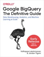
You can clone the repository corresponding to this book by clicking the Git icon (highlighted in Figure 5-4) and cloning https://github.com/GoogleCloudPlatform/bigquery-oreilly-book, as demonstrated in Figure 5-4.
Browse to and open the 05_devel/magics.ipynb notebook to try out the code in this section of the book. Change the PROJECT variable in the notebook to reflect your project. Then, on the menu at the top, select Run > Run All Cells.

Figure 5-4. Click the the Git icon (where the arrow is pointing) to clone a repository
Jupyter Magics
The BigQuery extensions for Jupyter make running queries within a notebook quite easy. For example, to run a query, you simply need to specify %%bigquery at the top of the cell:
%%bigquery --project $PROJECT
SELECT
  start_station_name
  , AVG(duration) as duration
  , COUNT(duration) as num_trips
FROM `bigquery-public-data`.london_bicycles.cycle_hire
GROUP BY start_station_name
ORDER BY num_trips DESC
LIMIT 5
Running a cell with this code executes the query and displays a nicely formatted table with the five desired rows, as shown in Figure 5-5.

Figure 5-5. The result of a query, nicely formatted, is embedded into the document
Running a parameterized query
To run a parameterized query, specify --params in the magic, as depicted in Figure 5-6. The parameters themselves are a Python variable that is typically defined elsewhere in the notebook.

Figure 5-6. How to run a parameterized query in a notebook
In the preceding example, the number of stations is a parameter that is specified as a Python variable and used in the SQL query to limit the number of rows in the result.
Saving query results to pandas
Saving the results of a query to pandas involves specifying the name of the variable (e.g., df) by which the pandas DataFrame will be referenced:
%%bigquery df --project $PROJECT
 SELECT
  start_station_name
  , AVG(duration) as duration
  , COUNT(duration) as num_trips
 FROM `bigquery-public-data`.london_bicycles.cycle_hire
 GROUP BY start_station_name
 ORDER BY num_trips DESC
You can use the variable df like any other pandas DataFrame. For example, we could ask for statistics of the numeric columns in df by using:
df.describe()
We can also use the plotting commands available in pandas to draw a scatter plot of the average duration of trips and the number of trips across all the stations, as presented in Figure 5-7.

Figure 5-7. Plotting a pandas DataFrame obtained by using a BigQuery query
Working with BigQuery, pandas, and Jupyter
We have introduced linkages between the Google Cloud Client Library for BigQuery and pandas in several sections of this book. Because pandas is the de facto standard for data analysis in Python, it might be helpful to bring together all of these capabilities and use them to illustrate a typical data science workflow.
Imagine that we are receiving anecdotes from our customer support team about bad bicycles at some stations. We’d like to send a crew out to spot-check a number of problematic stations. How do we choose which stations to spot-check? We could rely on stations from which we have received customer complaints, but we will tend to receive more complaints from busy stations simply because they have lots more customers.
We believe that if someone rents a bicycle for less than 10 minutes and returns the bicycle to the same station they rented it from, it is likely that the bicycle has a problem. Let’s call this a bad trip (from the customer’s viewpoint, it is). We could have our crew do a spot check of stations where bad trips have occurred more frequently.
To find the fraction of bad trips, we can query BigQuery using Jupyter Magics and save the result into a pandas DataFrame called badtrips using the following:
%%bigquery badtrips --project $PROJECT

WITH all_bad_trips AS (
SELECT
  start_station_name
  , COUNTIF(duration < 600 AND start_station_name = end_station_name) AS bad_trips
  , COUNT(*) as num_trips
FROM `bigquery-public-data`.london_bicycles.cycle_hire
WHERE EXTRACT(YEAR FROM start_date) = 2015
GROUP BY start_station_name
HAVING num_trips > 10
)
SELECT *, bad_trips / num_trips AS fraction_bad FROM all_bad_trips
ORDER BY fraction_bad DESC
The WITH expression counts the number of trips whose duration is less than 600 seconds and for which the starting and ending stations are the same. By grouping this by start_station_name, we get the total number of trips and bad trips at each station. The outer query computes the desired fraction and associates it with the station. This yields the following result (only the first few rows are shown):
start_station_name |
bad_trips |
num_trips |
fraction_bad |
|---|---|---|---|
| Contact Centre, Southbury House | 20 | 48 | 0.416667 |
| Monier Road, Newham | 1 | 25 | 0.040000 |
| Aberfeldy Street, Poplar | 35 | 955 | 0.036649 |
| Ormonde Gate, Chelsea | 315 | 8932 | 0.035266 |
| Thornfield House, Poplar | 28 | 947 | 0.029567 |
| ... |
It is clear that the station at the top of the table is quite odd. Just 48 trips originated from the Southbury House station, and 20 of those are bad! Nevertheless, we can confirm this by using pandas to look at the statistics of the DataFrame:
badtrips.describe()
This returns the following:
bad_trips |
num_trips |
fraction_bad |
|
|---|---|---|---|
| count | 823.000000 | 823.000000 | 823.000000 |
| mean | 75.074119 | 11869.755772 | 0.007636 |
| std | 70.512207 | 9906.268656 | 0.014739 |
| min | 0.000000 | 11.000000 | 0.000000 |
| 25% | 41.000000 | 5903.000000 | 0.005002 |
| 50% | 62.000000 | 9998.000000 | 0.006368 |
| 75% | 91.500000 | 14852.500000 | 0.008383 |
| max | 967.000000 | 95740.000000 | 0.416667 |
Examining the results, we notice that fraction_bad ranges from 0 to 0.417 (look at the min and max), but it is not clear how relevant this ratio is because the stations also vary quite dramatically. For example, the number of trips ranges from 11 to 95,740.
We can look at a scatter plot to see if there is any clear trend:
badtrips.plot.scatter('num_trips', 'fraction_bad');
Figure 5-8 displays the result.

Figure 5-8. In this plot, it seems that higher values of fraction_bad are associated with stations with low num_trips
It appears from the graph that higher values of fraction_bad are associated with stations with low num_trips, but the trend is not clear because of the outlier 0.4 value. Let’s zoom in a bit and add a line of best fit using the seaborn plotting package:
import seaborn as sns
ax = sns.regplot(badtrips['num_trips'],badtrips['fraction_bad']);
ax.set_ylim(0, 0.05);
As Figure 5-9 shows, this yields a clear depiction of the trend between the fraction of bad trips and how busy the station is.

Figure 5-9. It is clear that higher values of fraction_bad are associated with stations with low num_trips
Because higher values of fraction_bad are associated with stations with low num_trips, we should not have our crew simply visit stations with high values of fraction_bad. So, how should we choose a set of stations on which to conduct a spot check?
One approach could be to pick the five worst of the really busy stations, five of the next most busy, and so forth. We can do this by creating four different bands from the quantile of the stations by num_trips and then finding the five worst stations within each band. That’s what this pandas snippet does:
stations_to_examine = []
for band in range(1,5):
  min_trips = badtrips['num_trips'].quantile(0.2*(band))
  max_trips = badtrips['num_trips'].quantile(0.2*(band+1))
  query = 'num_trips >= {} and num_trips < {}'.format(
                                     min_trips, max_trips)
  print(query) # band
  stations = badtrips.query(query)
  stations = stations.sort_values(
                   by=['fraction_bad'], ascending=False)[:5]
  print(stations) # 5 worst
  stations_to_examine.append(stations)
  print()
The first band consists of the 20th to 40th percentile of stations by busyness:
num_trips >= 4826.4 and num_trips < 8511.8
                  start_station_name  bad_trips   num_trips  fraction_bad
6        River Street, Clerkenwell         221       8279      0.026694
9   Courland Grove, Wandsworth Road        105       5369      0.019557
10         Stanley Grove, Battersea         92       4882      0.018845
12              Southern Grove, Bow        112       6152      0.018205
18    Richmond Way, Shepherd's Bush        126       8149      0.015462
The last band consists of the 80th to 100th percentile of stations by busyness:
num_trips >= 16509.2 and num_trips < 95740.0
                      start_station_name bad_trips num_trips fraction_bad
25  Queen's Gate, Kensington Gardens        396      27457      0.014423
74     Speakers' Corner 2, Hyde Park        468      41107      0.011385
76        Cumberland Gate, Hyde Park        303      26981      0.011230
77            Albert Gate, Hyde Park        729      66547      0.010955
82      Triangle Car Park, Hyde Park        454      41675      0.010894
Notice that in the first band, it takes a fraction_bad of 0.015 to make the list, while in the last band, a fraction_bad of 0.01 is sufficient. The smallness of these numbers might make you complacent, but this is a 50% difference.
We can then use pandas to concatenate the various bands and the BigQuery API to write these stations back to BigQuery:
stations_to_examine = pd.concat(stations_to_examine)
bq = bigquery.Client(project=PROJECT)
tblref = TableReference.from_string(
                  '{}.ch05eu.bad_bikes'.format(PROJECT))
job = bq.load_table_from_dataframe(stations_to_examine, tblref)
job.result() # blocks and waits
We now have the stations to examine in a persistent storage, but we still need to get the data out to our crew. The best format for this is a map, and we can create it in Python if we know the latitude and longitude of our stations. We do, of course—the location of the stations is in the cycle_stations table:13
%%bigquery stations_to_examine --project $PROJECT
SELECT
  start_station_name AS station_name
  , num_trips
  , fraction_bad
  , latitude
  , longitude
FROM ch05eu.bad_bikes AS bad
JOIN `bigquery-public-data`.london_bicycles.cycle_stations AS s
ON bad.start_station_name = s.name
And here is the result (not all rows are shown):
station_name |
num_trips |
fraction_bad |
latitude |
longitude |
|---|---|---|---|---|
| Ormonde Gate, Chelsea | 8932 | 0.035266 | 51.487964 | -0.161765 |
| Stanley Grove, Battersea | 4882 | 0.018845 | 51.470475 | -0.152130 |
| Courland Grove, Wandsworth Road | 5369 | 0.019557 | 51.472918 | -0.132103 |
| Southern Grove, Bow | 6152 | 0.018205 | 51.523538 | -0.030556 |
| ... |
With the location information in hand, we can plot a map using the folium package:
import folium
map_pts = folium.Map(location=[51.5, -0.15], zoom_start=12)
for idx, row in stations_to_examine.iterrows():
  folium.Marker( location=[row['latitude'], row['longitude']],
                 popup=row['station_name'] ).add_to(map_pts)
This produces the beautiful interactive map shown in Figure 5-10, which our crew can use to check on the stations that we’ve identified.

Figure 5-10. An interactive map of the stations that need to be checked
We were able to seamlessly integrate BigQuery, pandas, and Jupyter to accomplish a data analysis task. We used BigQuery to compute aggregations over millions of bicycle rides, pandas to carry out statistical tasks, and Python packages such as folium to visualize the results interactively.
Working with BigQuery from R
Python is one of the most popular languages for data science, but it shares that perch with R, a long-standing programming language and software environment for statistics and graphics.
To use BigQuery from R, install the library bigrquery from CRAN:
install.packages("bigrquery", dependencies=TRUE)
Here’s a simple example of querying the bicycle dataset from R:
billing <- 'cloud-training-demos' # your project name
sql <- "
SELECT
  start_station_name
  , AVG(duration) as duration
    , COUNT(duration) as num_trips
  FROM `bigquery-public-data`.london_bicycles.cycle_hire
  GROUP BY start_station_name
  ORDER BY num_trips DESC
  LIMIT 5
"
tbl <- bq_project_query(billing, sql)
bq_table_download(tbl, max_results=100)
grid.tbl(tbl)
You use bq_project_query to create a BigQuery query, and you execute it by using bq_table_download.
You can also use R from a Jupyter notebook. The conda environment for Jupyter14 has an R extension that you can load by running the following:
!conda install rpy2
%load_ext rpy2.ipython
To carry out a linear regression to predict the number of docks at a station based on its location, you can first populate an R DataFrame from BigQuery:
%%bigquery docks --project $PROJECT
SELECT
  docks_count, latitude, longitude
FROM `bigquery-public-data`.london_bicycles.cycle_stations
WHERE bikes_count > 0
Then Jupyter Magics for R can be performed just like the Jupyter Magics for Python. Thus, you can use the R magic to perform linear modeling (lm) on the docks DataFrame:
%%R -i docks
mod <- lm(docks ~ latitude + longitude)
summary(mod)
Cloud Dataflow
We introduced Cloud Dataflow in Chapter 4 as a way to load data into BigQuery from MySQL. Cloud Dataflow is a managed service for executing pipelines written using Apache Beam. Dataflow is quite useful in data science because it provides a way to carry out transformations that would be difficult to perform in SQL. As of this writing, Beam pipelines can be written in Python, Java, and Go, with Java the most mature.
As an example of where this could be useful, consider the distribution of the length of bicycle rentals from an individual bicycle station shown in Figure 5-11.

Figure 5-11. Distribution of the duration of bicycle rides from a single station
As Figure 5-11 demonstrates, because the bar at x = 1000 has y = 1500, there were approximately 1,500 rides that were around 1,000 seconds in duration.
Although the specific durations are available in the BigQuery table, it can be helpful to fit these values to a theoretical distribution so that we can carry out simulations and study the effect of pricing and availability changes more readily. In Python, given an array of duration values, it is quite straightforward to compute the parameters of a Gamma distribution fit using the scipy package:
from scipy import stats
ag,bg,cg = stats.gamma.fit(df['duration'])
Imagine that you want to go through all of the stations and compute the parameters of the Gamma distribution fit to the duration of rentals from each of those stations. Because this is not convenient in SQL but can easily be done in Python, we can write a Dataflow job to compute the Gamma fits in a distributed manner—that is, to parallelize the computation of Gamma fits on a cluster of machines.
The pipeline starts with a query15 to pull the durations for each station, sends the resulting rows to the method compute_fit, and then writes the resulting rows to BigQuery, to the table station_stats:16
  opts = beam.pipeline.PipelineOptions(flags = [], **options)
  RUNNER = 'DataflowRunner'
  query = """
       SELECT start_station_id, ARRAY_AGG(duration) AS duration_array
       FROM `bigquery-public-data.london_bicycles.cycle_hire`
       GROUP BY start_station_id
       """

  with beam.Pipeline(RUNNER, options = opts) as p:
     (p
       | 'read_bq' >> beam.io.Read(beam.io.BigQuerySource(query=query))
       | 'compute_fit' >> beam.Map(compute_fit)
       | 'write_bq' >> beam.io.gcp.bigquery.WriteToBigQuery(
           'ch05eu.station_stats',
schema='station_id:string,ag:FLOAT64,bg:FLOAT64,cg:FLOAT64')
    )
The compute_fit method is a Python function that takes in a dictionary corresponding to the input BigQuery row and returns a dictionary corresponding to the desired output row:
def compute_fit(row):
  from scipy import stats
  result = {}
  result['station_id'] = row['start_station_id']
  durations = row['duration_array']
  ag, bg, cg = stats.gamma.fit(durations)
  result['ag'] = ag
  result['bg'] = bg
  result['cg'] = cg
  return result
The fit values are then written to a destination table.
After launching the Dataflow job, we can monitor it via the GCP Cloud Console, shown in Figure 5-12, and see the job autoscaling to process the stations in parallel.

Figure 5-12. The Dataflow job is parallelized and run on a cluster whose size is autoscaled based on the rate of progress in each step
When the Dataflow job finishes, we can query the table and obtain statistics of the stations and plot the parameters of the Gamma distribution (see the notebook on GitHub for the graphs).
JDBC/ODBC drivers
Because BigQuery is a warehouse for structured data, it can be convenient if database-agnostic APIs like Java Database Connectivity (JDBC) and Open Database Connectivity (ODBC) can be employed by a Java or .NET application to communicate with a BigQuery database driver. This is not recommended for new applications—use the client library instead. If, however, you have a legacy application that communicates with a database today and needs to be converted with minimal code changes to communicate with BigQuery, the use of a JDBC/ODBC driver might be warranted.
Warning
We strongly recommend the use of the client libraries (in the language of your choice) over the use of JDBC/ODBC drivers because the functionality exposed by the JDBC/ODBC driver is a subset of the full capabilities of BigQuery. Among the features missing are support for large-scale ingestion (i.e., many of the loading techniques described in the previous chapter), large-scale export (meaning data movement will be slow), and nested/repeated fields (preventing the use of many of the performance optimizations that we cover in Chapter 7). Designing new systems based on JDBC/ODBC drivers tends to lead to painful technical debt.
A Google partner does provide ODBC and JDBC drivers capable of executing BigQuery Standard SQL queries.17 To install the Java drivers, for example, you would download a ZIP file, unzip it, and place all of the Java Archive (JAR) files in the ZIP folder in the classpath of your Java application. Using the driver in a Java application typically involves modifying a configuration file that specifies the connection information. There are several options to configure the authentication and create a connection string that can be used within your Java application.
Incorporating BigQuery Data into Google Slides (in G Suite)
It is possible to use Google Apps Script to manage BigQuery projects, upload data, and execute queries. This is useful if you want to automate the population of Google Docs, Google Sheets, or Google Slides with BigQuery data.
As an example, let’s look at creating a pair of slides with analysis of the London bicycles data. Begin by going to https://script.google.com/create to create a new script. Then, on the Resources menu, choose Advanced Google Services and flip on the bit for the BigQuery API (name the project if prompted).
The full Apps Script for this example is in the GitHub repository for this book, so copy the script and paste it into the text editor. Then, at the top of the script, change the PROJECT_ID, choose the function createBigQueryPresentation, and then click the run button, as illustrated in Figure 5-13.

Figure 5-13. Use Google Apps Script to create a presentation from data in BigQuery
The resulting spreadsheet and slide deck will show up in Google Drive (you can also find their URLs by clicking View > Logs). The slide deck will look similar to that shown in Figure 5-14.

Figure 5-14. Slide deck created by the Google Apps Script
The function createBigQueryPresentation carried out the following code:
function createBigQueryPresentation() {
  var spreadsheet = runQuery();
  Logger.log('Results spreadsheet created: %s', spreadsheet.getUrl());
  var chart = createColumnChart(spreadsheet); // UPDATED
  var deck = createSlidePresentation(spreadsheet, chart); // NEW
  Logger.log('Results slide deck created: %s', deck.getUrl()); // NEW
}
Essentially, it calls three functions:
-
runQueryto run a query and store the results in a Google Sheets spreadsheet -
createColumnChartto create a chart from the data in the spreadsheet -
createSlidePresentationto create the output Google Slides slide deck
The runQuery() method uses the Apps Scripts client library to invoke BigQuery and page through the results:
var queryResults = BigQuery.Jobs.query(request, PROJECT_ID);
var rows = queryResults.rows;
  while (queryResults.pageToken) {
     queryResults = BigQuery.Jobs.getQueryResults(PROJECT_ID, jobId, {
       pageToken: queryResults.pageToken
     });
     rows = rows.concat(queryResults.rows);
  }
Then it creates a spreadsheet and adds these rows to the sheet. The other two functions employ Apps Scripts code to draw graphs, create a slide deck, and add both types of data to the slide deck.
Bash Scripting with BigQuery
The bq command-line tool that is provided as part of the Google Cloud Software Development Kit (SDK) provides a convenient way to invoke BigQuery operations from the command line. The SDK is installed by default on Google Cloud virtual machines (VMs) and clusters. You can also download and install the SDK in your on-premises development and production environments.
You can use the bq tool to interact with the BigQuery service when writing Bash scripts or by calling out to the shell from many programming languages without the need to depend on the client library. Common uses of bq include creating and verifying the existence of datasets and tables, executing queries, loading data into tables, populating tables and views, and verifying the status of jobs. Let’s look at each of these.
Creating Datasets and Tables
To create a dataset, use bq mk and specify the location of the dataset (e.g., US or EU). It is also possible to specify nondefault values for such things as the table expiration time. It is a best practice to provide a description for the dataset:
bq mk --location=US
      --default_table_expiration 3600
      --description "Chapter 5 of BigQuery Book."
      ch05
Checking whether a dataset exists
The bq mk in the preceding example fails if the dataset already exists. To create the dataset only if the dataset doesn’t already exist, you need to list existing datasets using bq ls and check whether that list contains a dataset with the name you’re looking for:18
#!/bin/bash
 bq_safe_mk() {
     dataset=$1
     exists=$(bq ls --dataset | grep -w $dataset)
     if [ -n "$exists" ]; then
        echo "Not creating $dataset since it already exists"
     else
        echo "Creating $dataset"
        bq mk $dataset
     fi
}
# this is how you call the function
bq_safe_mk ch05
Creating a dataset in a different project
The dataset ch05 is created in the default project (specified when you logged into the VM or when you ran gcloud auth using the Google Cloud SDK). To create a dataset in a different project, qualify the dataset name with the name of the project in which the dataset should be created:
bq mk --location=US
       --default_table_expiration 3600
       --description "Chapter 5 of BigQuery Book."
       projectname:ch05
Creating a table
Creating a table is similar to creating a dataset except that you must add --table to the bq mk command. The following creates a table named ch05.rentals_last_hour that expires in 3,600 seconds and that has two columns named rental_id (a string) and duration (a float):
bq mk --table
    --expiration 3600
    --description "One hour of data"
     --label persistence:volatile
     ch05.rentals_last_hour rental_id:STRING,duration:FLOAT
You can use the label to tag tables with characteristics; Data Catalog supports the ability to search for tables that have a specific label—here, persistence is the key and volatile is the label.
Complex schema
For more complex schemas that cannot easily be expressed by a comma-separated string, specify a JSON file, as explained in Chapter 4:
bq mk --table
    --expiration 3600
    --description "One hour of data"
     --label persistence:volatile
     ch05.rentals_last_hour schema.json
Copying datasets
The most efficient way to copy datasets is through the command-line tool. For example, this copies a table from the ch04 dataset to the ch05 dataset:
bq cp ch04.old_table ch05.new_table
Tip
Copying tables can take a while, but your script might not be able to proceed until the job is complete. An easy way to wait for a job to complete is to use bq wait:
bq wait --fail_on_error job_id
This preceding code waits forever until the job completes, whereas the following waits a maximum of 600 seconds:
bq wait --fail_on_error job_id 600
If there is only one running job, you can omit the job_id.
Loading and inserting data
We covered loading data into a destination table using bq load rather exhaustively in Chapter 4. For a refresher, see that chapter.
To insert rows into a table, write the rows as newline-delimited JSON and use bq insert:
bq insert ch05.rentals_last_hour data.json
In this example, the file data.json contains entries corresponding to the schema of the table being inserted into the following:
{"rental_id":"345ce4", "duration":240}
Executing Queries
To execute a query, use bq query and specify the query:
bq query
     --use_legacy_sql=false
     'SELECT MAX(duration) FROM
     `bigquery-public-data`.london_bicycles.cycle_hire'
You also can provide the query string via the standard input:
echo "SELECT MAX(duration) FROM
`bigquery-public-data`.london_bicycles.cycle_hire"
| bq query --use_legacy_sql=false
Providing the query in a single string and escaping quotes and so on can become quite cumbersome. For readability, use the ability of Bash to read a multiline string into a variable:19
#!/bin/bash
read -d '' QUERY_TEXT << EOF
SELECT
  start_station_name
  , AVG(duration) as duration
  , COUNT(duration) as num_trips
FROM `bigquery-public-data`.london_bicycles.cycle_hire
GROUP BY start_station_name
ORDER BY num_trips DESC
LIMIT 5
EOF
bq query --project_id=some_project --use_legacy_sql=false $QUERY_TEXT
In this code, we are reading into the variable QUERY_TEXT a multiline string that will be terminated by the word EOF. We can then pass that variable into bq query.
The preceding code is also an illustration of explicitly specifying the project that is to be billed for the query.
Remember to use --use_legacy_sql=false, because the default dialect used by bq is not the Standard SQL that we cover in this book!
Previewing data
To preview a table, use bq head. Unlike a query of SELECT * followed by LIMIT, this is deterministic and doesn’t incur BigQuery charges.
To view the first 10 rows, you can do the following:
bq head -n 10 ch05.bad_bikes
To view the next 10 rows, do this:
bq head -s 10 -n 10 ch05.bad_bikes
Note that the table is not actually ordered, and so you should treat this as a way to read an arbitrary set of rows.
Creating views
You can create views and materialized views from queries using bq mk. For example, this creates a view named rental_duration in the dataset ch05:
#!/bin/bash
read -d '' QUERY_TEXT << EOF
SELECT
  start_station_name
  , duration/60 AS duration_minutes
FROM `bigquery-public-data`.london_bicycles.cycle_hire
EOF
bq mk --view=$QUERY_TEXT ch05.rental_duration
Views in BigQuery can be queried just like tables, but they act like subqueries—querying a view will bring the full text of the view into the calling query. Materialized views save the query results of the view into a table that is then queried. BigQuery takes care of ensuring that the materialized view is up to date. We cover views and materialized views in more detail in Chapter 10. To create a materialized view, replace --view in the preceding snippet with --materialized_view.
BigQuery Objects
We looked at bq ls --dataset as a way to list the datasets in a project. As Table 5-3 demonstrates, there are other things you can list as well.
| Command | What it lists |
|---|---|
bq ls ch05 |
Tables in the dataset ch05 |
bq ls -p |
All projects |
bq ls -j some_project |
All the jobs in the specified project |
bq ls --dataset |
All the datasets in the default project |
bq ls --dataset some_project |
All the datasets in the specified project |
bq ls --models |
Machine learning models |
bq ls --transfer_run --filter='states:PENDING' --run_attempt='LATEST' projects/p/locations/l /transferConfigs/c |
Transfer runs filtered to show only pending ones |
bq ls --reservation_grant --project_id=some_proj --location='us' |
Reservation grants for slots in the specified project |
Showing details
Table 5-4 illustrates how you can look at the details of a BigQuery object using bq show.
| Command | Details of this object are shown |
|---|---|
bq show ch05 |
The dataset ch05 |
bq show -j some_job_id |
The specified job |
bq show --schema ch05.bad_bikes |
The schema of the table ch05.bad_bikes |
bq show --view ch05.some_viewbq show --materialized_view ch05.some_view |
The specified view |
bq show --model ch05.some_model |
The specified model |
bq show --transfer_run projects/p/locations/l/transferConfigs/c/runs/r |
The transfer run |
In particular, note that you can list jobs using bq ls and verify the status of jobs using bq show.
Updating
You can update the details of already created tables, datasets, and so on using bq update:
bq update --description "Bikes that need repair" ch05.bad_bikes
You can use bq update to update the query corresponding to a view or materialized view,
bq update
   --view "SELECT ..."
   ch05.rental_duration
and even the size of a reservation (we will look at slots and reservations in Chapter 6):
bq update --reservation --location=US
          --project_id=some_project
          --reservation_size=2000000000
Summary
In this chapter, we looked at three different forms of BigQuery client libraries:
-
A REST API that can be accessed from programs written in any language that can communicate with a web server
-
A Google API client that uses autogenerated language bindings in many programming languages
-
A custom-built BigQuery client library that provides a convenient way to access BigQuery from a number of popular programming languages
Of these, the recommended approach is to use the BigQuery client library, provided one is available for your language of choice. If a BigQuery client library doesn’t exist, use the Google API client. Only if you are working in an environment in which even the API client is not available should you interact with the REST API directly.
There are a couple of higher-level abstractions available that make programming against BigQuery easy in two commonly used environments: Jupyter notebooks and shell scripts. We delved into the support for BigQuery from Jupyter and pandas and illustrated how the combination of these tools provides a powerful and extensible environment for sophisticated data science workflows. We also touched on integration with R and with G Suite and covered many of the capabilities of the bq command-line tool. Finally, we covered Bash scripting with BigQuery.
1 Other APIs, especially non-REST APIs such as gRPC ones, will have a different API prefix.
2 Specifically, https://www.googleapis.com/auth/bigquery or https://www.googleapis.com/auth/cloud-platform have to be allowed.
3 This is the file 05_devel/rest_list.sh in the GitHub repository for this book. You can run it anywhere that you have the Cloud SDK and curl installed (such as in Cloud Shell). Because we have not created it in this chapter yet, I’m using the dataset (ch04) that we loaded in the previous chapter.
4 See 05_devel/rest_query.sh in the GitHub repository for this book.
5 See 04_devel/rest_query_async.sh in the GitHub repository for this book.
6 This requires the pyarrow library. If you don’t have it already, install it by using pip install pyarrow.
7 Because pandas, by default, alphabetizes the column names, your BigQuery table will have a schema that is alphabetized and not in the order in which the column names appear in the tuples.
8 For the full set of support URIs, see https://cloud.google.com/bigquery/docs/reference/rest/v2/jobs#configuration.load.sourceUris.
9 To create a bucket in the EU region, use: gsutil mb -l EU gs://some-bucket-name.
10 Which five rows we get will be arbitrary because BigQuery does not guarantee ordering. The purpose of providing the start_index is so that we can get the “next page” of five rows by supplying start_index=5.
11 This is the same API used by the BigQuery web UI to show you the estimate.
12 This is the script 05_devel/launch_notebook.sh in the GitHub repository for this book.
13 This is the point of data warehousing: to bring enterprise data together into a centralized repository so that any enterprise data that an analyst might possibly need is only a join away.
14 As of this writing, the PyTorch image for the Notebook Instance on GCP is built using conda.
15 These queries are billed as part of the Dataflow job.
16 See 05_devel/statfit.ipynb in the GitHub repository for this book.
17 See https://cloud.google.com/bigquery/partners/simba-drivers/ and https://www.simba.com/drivers/bigquery-odbc-jdbc/.
18 This is, of course, subject to race conditions if someone else created the dataset between your check and actual creation.
19 See 05_devel/bq_query.sh in the GitHub repository for this book.