What Can a QPU Do for Computer Graphics?

In this chapter we explore one particular QIP application called Quantum Supersampling (QSS). QSS leverages a QPU to find intriguing improvements to the computer graphics task of supersampling, as is summarized in Figure 11-1. Supersampling is a conventional computer graphics technique whereby an image generated by a computer at high resolution is reduced to a lower-resolution image by selectively sampling pixels. Supersampling is an important step in the process of producing usable output graphics from computer-generated images.

QSS was originally developed as a way to speed up supersampling with a QPU, and by this metric it failed. However, numerical analysis of the results revealed something interesting. Although the final image quality of QSS (measured as error per pixel) is about the same as for existing conventional methods, the output image has a different kind of advantage.

Figure 11-1. Results of QSS (with ideal and conventional cases for comparison); these reveal a change in the character of the noise in a sampled image

Figure 11-1 shows that the average pixel noise¹ in the conventional and QSS sampled images is about the same, but the character of the noise is very different. In the conventionally sampled image, each pixel is a little bit noisy. In the quantum image, some of the pixels are very noisy (black and white specks), while the rest are perfect.

Imagine you’ve been given an image, and you’re allowed 15 minutes to manually remove the visible noise. For the image generated by QSS the task is fairly easy; for the conventionally sampled image, it’s nearly impossible.

QSS combines a range of QPU primitives: quantum arithmetic from Chapter 5, amplitude amplification from Chapter 6, and the Quantum Fourier Transform from Chapter 7. To see how these primitives are utilized, we first need a little more background in the art of supersampling.

Conventional Supersampling

Ray tracing_ is a technique for producing computer-generated images, where increased computational resources allow us to produce results of increasing quality. Figure 11-2 shows a schematic representation of how ray tracing produces images from computer-generated scenes.

Figure 11-2. In ray tracing, many samples are taken for each pixel of the final image

For each pixel in the final image, a mathematical ray is projected in 3D space from the camera through the pixel and toward the computer-generated scene. The ray strikes an object in the scene, and in the simplest version (ignoring reflections and transparency) the object’s color determines the color of the corresponding pixel in the image.

While casting just one ray per pixel would produce a correct image, for faraway details such as the tree in Figure 11-2 edges and fine details in the scene are lost. Additionally, as the camera or the object moves, troublesome noise patterns appear on objects such as tree leaves and picket fences.

To solve this without making the image size ridiculously large, ray-tracing software casts multiple rays per pixel (hundreds or thousands is typical) while varying the direction slightly for each one. Only the average color is kept, and the rest of the detail is discarded. This process is called supersampling, or Monte Carlo sampling. As more samples are taken, the noise level in the final image is reduced.

Supersampling is a task where we perform parallel processing (calculating the results of many rays interacting with a scene), but ultimately only need the sum of the results, not the individual results themselves. This sounds like something a QPU might help with! A full QPU-based ray-tracing engine would require far more qubits than are currently available. However, to demonstrate QSS we can use a QPU to draw higher-resolution images by less-sophisticated methods (ones not involving ray-tracing!), so that we can study how a QPU impacts the final resolution-reducing supersampling step.

Hands-on: Computing Phase-Encoded Images

To make use of a QPU for supersampling, we’ll need a way of representing images in a QPU register (one that isn’t as tricky as full-blown ray tracing!).

There are many different ways to represent pixel images in QPU registers and we summarize a number of approaches from the quantum image processing literature at the end of this chapter. However, we’ll use a representation that we refer to as phase encoding, where the values of pixels are represented in the phases of a superposition. Importantly, this allows our image information to be compatible with the amplitude amplification technique we introduced in Chapter 6.

Figure 11-3. Ce n’est pas une mouche²

In this chapter we’ll learn how phase-encoded images like this can be created, and then use them to demonstrate Quantum Supersampling.

A QPU Pixel Shader

A pixel shader is a program (often run on a GPU) that takes an x and y position as input, and produces a color (black or white in our case) as output. To help us demonstrate QSS, we’ll construct a quantum pixel shader.

To begin, Example 11-1 initializes two four-qubit registers, qx and qy. These will serve as the x and y input values for our shader. As we’ve seen in previous chapters, performing a HAD on all qubits produces a uniform superposition of all possible values, as in Figure 11-4. This is our blank canvas, ready for drawing.

Figure 11-4. A blank quantum canvas

Using PHASE to Draw

Now we’re ready to draw. Finding concise ways to draw into register phases can get complicated and subtle, but we can start by filling the right half of the canvas simply by performing the operation “if qx >= 8 then invert phase.” This is accomplished by applying a PHASE(180) to a single qubit, as demonstrated in Figure 11-5:

// Set up and clear the canvas
qc.reset(8);
var qx = qint.new(4, 'qx');
var qy = qint.new(4, 'qy');
qc.write(0);
qx.hadamard();
qy.hadamard();

// Invert if qx >= 8
qc.phase(180, qx.bits(0x8));

Figure 11-5. Phase-flipping half of the image

Note

In a sense, we’ve used just one QPU instruction to fill 128 pixels. On a GPU, this would have required the pixel shader to run 128 times. As we know only too well, the catch is that if we try to READ the result we get only a random value of qx and qy.

With a little more logic, we can fill a square with a 50% gray dither pattern.⁴ For this, we want to flip any pixels where qx and qy are both greater than or equal to 8, and where the low qubit of qx is not equal to the low qubit of qy. We do this in Example 11-1, and the results can be seen in Figure 11-6.

Figure 11-6. Adding a dither pattern

With a little arithmetic from Chapter 5, we can create more interesting patterns, as shown in Figure 11-7:

// Clear the canvas
qc.reset(8);
var qx = qint.new(4, 'qx');
var qy = qint.new(4, 'qy');
qc.write(0);
qx.hadamard();
qy.hadamard();

// fun stripes
qx.subtractShifted(qy, 1);
qc.phase(180, qx.bits(0x8));
qx.addShifted(qy, 1);

Figure 11-7. Playing with stripes

Drawing Curves

To draw more complex shapes, we need more complex math. Example 11-2 demonstrates the use of the addSquared() QPU function from Chapter 5 to draw a quarter-circle with a radius of 13 pixels. The result is shown in Figure 11-8. In this case, the math must be performed in a larger 10-qubit register, to prevent overflow when we square and add qx and qy. Here we’ve used the trick learned in Chapter 10 of storing the value of a logical (or mathematical) operation in the phase of a state, through a combination of magnitude and phase-logic operations.

Figure 11-8. Drawing curves in Hilbert space

If the qacc register is too small, the math performed in it will overflow, resulting in curved bands. This overflow effect will be used deliberately in Figure 11-11, later in the chapter.

Sampling Phase-Encoded Images

Now that we can represent images in the phases of quantum registers, let’s return to the problem of supersampling. Recall that in supersampling we have many pieces of information calculated from a computer-generated scene (corresponding to different rays we have traced) that we want to combine to give a single pixel in our final output image. software verification To simulate this, we can consider our 16×16 array of quantum states to be made of 16 4×4 tiles as shown in Figure 11-9.

We imagine that the full 16×16 image is the higher-resolution data, which we then want reduce into 16 final pixels.

Since they’re only 4×4 subpixels, the qx and qy registers needed to draw into these tiles can be reduced to two qubits each. We can use an overflow register (which we call qacc since such registers are often referred to as accumulators) to perform any required logical operations that won’t fit in two qubits. Figure 11-10 (Example 11-3) shows the circuit for performing the drawing shown in Figure 11-9, tile by tile.

Note that in this program, the variables tx and ty are digital values indicating which tile of the image the shader is working on. We get the absolute x value of a subpixel that we want to draw by adding qx and (tx x 4), which we can easily compute since tx and ty are not quantum. Breaking our images into tiles this way makes it easier for us to subsequently perform supersampling.

Figure 11-9. A simple image divided into subpixels

Figure 11-10. Drawing the subpixels of one tile in superposition

A More Interesting Image

With a more sophisticated shader program, we can produce a more interesting test for the quantum supersampling algorithm. In order to test and compare supersampling methods, here we use circular bands to produce some very high-frequency detail. The full source code for the image in Figure 11-11, which also splits the phase-encoded image into tiles as we mentioned earlier, can be run at http://oreilly-qc.github.io?p=11-A.

×

Figure 11-11. A more involved image with some high-frequency detail conventionally rendered at 256×256 pixels (shown here).

Now that we have a higher-resolution phase-encoded image broken up into tiles, we’re ready to apply the QSS algorithm. In this case, the full image is drawn at 256×256 pixels. We’ll use 4,096 tiles, each composed of 4×4 subpixels, and supersample all the subpixels in a single tile to generate one pixel of the final sampled image from its 16 subpixels.

Supersampling

For each tile, we want to estimate the number of subpixels that have been phase-flipped. With black and white subpixels (represented for us as flipped or unflipped phases), this allows us to obtain a value for each final pixel representative of the intensity of its original constituent subpixels. Handily, this problem is exactly the same as the Quantum Sum Estimation problem from “Multiple Flipped Entries”.

To make use of Quantum Sum Estimation, we simply consider the quantum program implementing our drawing instructions to be the flip subroutine we use in amplitude amplification from Chapter 6. Combining this with the Quantum Fourier Transform from Chapter 7 allows us to approximate the total number of flipped subpixels in each tile. This involves running our drawing program multiple times for each tile.

Note that, without a QPU, sampling a high-resolution image into a lower-resolution one would still require running a drawing subroutine multiple times for each tile, randomizing the values qx and qy for each sample. Each time we would simply receive a “black” or “white” sample, and by adding these up we would converge on an approximated image.

The sample code in Example 11-4 shows the results of both quantum and conventional supersampling (typically performed in the conventional case by a technique known as Monte Carlo sampling), and we see them compared in Figure 11-12. The ideal reference shows the result we would get from perfect sampling, and the QSS lookup table is a tool we discuss in detail in the coming pages.

Figure 11-12. Comparison of quantum and conventional supersampling

As mentioned at the beginning of this chapter, the interesting advantage we obtain with QSS is not to do with the number of drawing operations that we have to perform, but rather relates to a difference in the character of the noise we observe.

In this example, when comparing equivalent numbers of samples, QSS has about 33% lower mean pixel error than Monte Carlo. More interestingly, the number of zero-error pixels (pixels in which the result exactly matches the ideal) is almost double that of the Monte Carlo result.

QSS Versus Conventional Monte Carlo Sampling

In contrast to conventional Monte Carlo sampling, our QSS shader never actually outputs a single subpixel value. Instead, it uses the superposition of possible values to estimate the sum you would have gotten from calculating them all and adding them up. If you actually need to calculate every subpixel value along the way, then a conventional computing approach is a better tool for the job. If you need to know the sum, or some other characteristic of groups of subpixels, a QPU offers an interesting alternative approach.

The fundamental difference between QSS and conventional supersampling can be characterized as follows:

Conventional supersampling

As the number of samples increases, the result converges toward the exact answer.

Quantum supersampling

As the number of samples increases, the probability of getting the exact answer increases.

Now that we have an idea of what QSS can do for us, let’s expand a little on how it works.

How QSS Works

The core idea behind QSS is to use the approach we first saw in “Multiple Flipped Entries”, where combining amplitude amplification iterations with the Quantum Fourier Transform (QFT) allows us to estimate the number of items flipped by whatever logic we use in the flip subroutine of each AA iteration.

In the case of QSS, flip is provided by our drawing program, which flips the phase of all of the “white” subpixels.

We can understand the way that AA and QFT and work together to help us count flipped items as follows. First, we perform a single AA iteration conditional on the value of a register of “counter” qubits. We call this register a “counter” precisely because its value determines how many AA iterations our circuit will perform. If we now use HAD operations to prepare our counter register in superposition we will be performing a superposition of different numbers of AA iterations. Recall from “Multiple Flipped Entries” that the READ probabilities for multiple flipped values in a register are dependent on the number of AA iterations that we perform. We noted in this earlier discussion that oscillations are introduced depending on the number of flipped values. Because of this, when we perform a superposition of different numbers of AA iterations, we introduce a periodic oscillation across the amplitudes of our QPU register having a frequency that depends on the number of flipped values.

When it comes to READing frequencies encoded in QPU registers, we know that the QFT is the way to go: using the QFT we can determine this frequency, and consequently the number of flipped values (i.e., number of shaded subpixels). Knowing the number of subpixels we’ve supersampled for a single pixel in our final lower-resolution image, we can then use this to determine the brightness we should use for that pixel.

Although this might be a little difficult to parse in text on a page, stepping through the code in Example 11-4 and inspecting the resulting circle notation visualizations will hopefully make the approach taken by QSS more apparent.

Note that the more counter qubits we use, the better the sampling of the image will be, but at the cost of having to run our drawing code more times. This trade-off is true for both quantum and conventional approaches, as can be seen in Figure 11-13.

Figure 11-13. Increasing the number of iterations

The QSS lookup table

When we run the QSS algorithm and finish by READing out our QPU register, the number we get will be related but not directly equal to the number of white pixels within a given tile.

The QSS lookup table is the tool we need to look up how many subpixels a given READ value implies were within a tile. The lookup table needed for a particular image doesn’t depend on the image detail (or more precisely, the details of the quantum pixel shader we used). We can generate and reuse a single QSS lookup table for any QSS applications having given tile and counter register sizes.

For example, Figure 11-14 shows a lookup table for QSS applications having a 4×4 tile size and a counter register consisting of four qubits.

Figure 11-14. The QSS lookup table is used to translate QSS results into sampled pixel brightness

The rows (y-axis) of the lookup table enumerate the possible outcomes we might read in the output QPU register from an application of QSS. The columns (x-axis) enumerate the different possible numbers of subpixels within a tile that could lead to these READ values. The grayscale colors in the table graphically represent the probabilities associated with the different possible READ values (lighter colors here denoting higher probabilities). Here’s an example of how we could use the lookup table. Suppose we read a QSS result of 10. Finding that row in the QSS lookup table, we see that this result most likely implies that we have supersampled five white subpixels. However, there’s also a nonzero probability we supersampled four or six (or to a lesser extent three or seven) subpixels. Note that some error is introduced as we cannot always uniquely infer the number of sampled subpixels from a READ result.

Such a lookup table is used by the QSS algorithm to determine a final result. How do we get our hands on a QSS lookup table for a particular QSS problem? The code in Example 11-5 shows how we can calculate the QSS lookup table. Note that this code doesn’t rely on a particular quantum pixel shader (i.e., particular image). Since the lookup table only associated the READ value with a given number of white subpixels per tile (regardless of their exact locations), it can be generated without any knowledge of the actual image to be supersampled.

The QSS lookup table tells us a lot about how QSS performs for given counter register and tile sizes, acting as a sort of fingerprint for the algorithm. Figure 11-15 shows a few examples of how the lookup table changes as (for a fixed counter register size of four qubits) we increase the tile size (and therefore number of subpixels) used in our QSS algorithm.

Figure 11-15. Increasing the number of subpixels adds columns

Similarly, Figure 11-16 shows how the lookup table changes as we increase the number of counter qubits used (for a given tile size).

Figure 11-16. Increasing the counter size adds rows

Confidence maps

In addition to being a tool for interpreting READ values, we can also use a QSS lookup table to evaluate how confident we are in the final brightness of a pixel. By looking up a given pixel’s QSS READ value in a row of the table, we can judge the probability that a pixel value we’ve inferred is correct. For example, in the case of the lookup table in Figure 11-14, we’d be very confident of values READ to be 0 or 1, but much less confident if we’d READ values of 2, 3, or 4. This kind of inference can be used to produce a “confidence map” indicating the likely locations of errors in images we produce with QSS, as illustrated in Figure 11-17.

Figure 11-17. QSS result and associated confidence map generated from a QSS lookup table—in the confidence map brighter pixels denote areas where the result is more likely correct

Adding Color

The images we’ve been rendering with QSS in this chapter have all been one-bit monochrome, using flipped QPU register phases to represent black and white pixels. Although we’re big fans of retro gaming, perhaps we can incorporate a few more colors? We could simply use the phases and amplitudes of our QPU register to encode a wider range of color values for our pixels, but then the Quantum Sum Estimation used by QSS would no longer work.

However, we can borrow a technique from early graphics cards known as bitplanes. In this approach we use our quantum pixel shader to render separate monochrome images, each representing one bit of our image. For example, suppose we want to associate three colors with each pixel in our image (red, green, and blue). Our pixel shader can then essentially generate three separate monochrome images, each of which represents the contribution of one of the three color channels. These three images can undergo supersampling separately, before being recombined into a final color image.

This only allows us eight colors (including black and white); however, supersampling allows us to blend subpixels together, effectively producing a 12-bit-per-pixel image (see Figure 11-18). The complete code for this can be found at http://oreilly-qc.github.io?p=11-6.

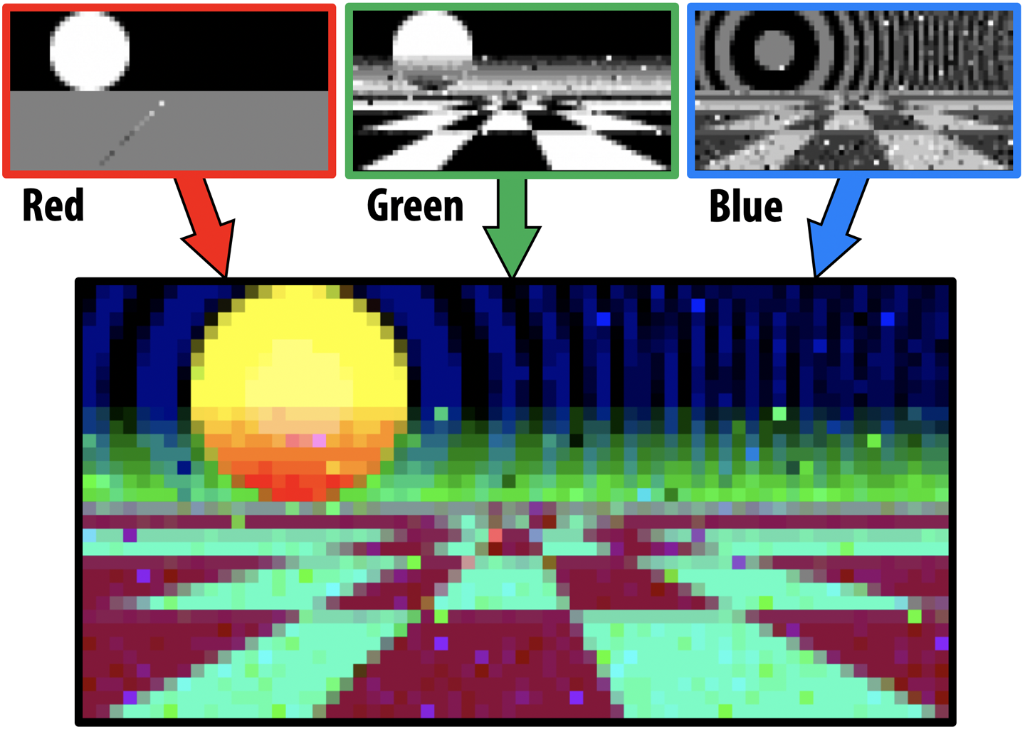
Figure 11-18. Combining supersampled color planes. Space Harrier eat your heart out!

Conclusion

This chapter demonstrated how exploring new combinations of QPU primitives with a little domain knowledge can potentially lead to new QPU applications. The ability to redistribute sampling noise also shows visually how sometimes we have to look beyond speedups to see the advantages of QPU applications.

It’s also worth noting that the ability of Quantum Supersampling to produce novel noise redistributions potentially has relevance beyond computer graphics. Many other applications also make heavy use of Monte Carlo sampling, in fields such as artificial intelligence, computational fluid dynamics, and even finance.

To introduce Quantum Supersampling, we used a phase encoding representation of images in QPU registers. It is worth noting that Quantum Image Processing researchers have also proposed many other such representations. These include the so-called Qubit Lattice representation,⁵ Flexible Representation of Quantum Images (FRQI),⁶ Novel Enhanced Quantum Representation (NEQR),⁷ and Generalized Quantum Image Representation (GQIR).⁸ These representations⁹ have been used to explore other image processing applications including template matching,¹⁰ edge detection,¹¹ image classification,¹² and image translation¹³ to name but a few.¹⁴