Chapter 10. Quantum Search
In Chapter 6 we saw how the amplitude amplification (AA) primitive changes differences in phases within a register into detectable variations in magnitude. Recall that when introducing AA, we assumed that applications would provide a subroutine to flip the phases of values in our QPU register. As a simplistic example, we used the flip circuit as a placeholder, which simply flipped the phase of a single known register value. In this chapter we will look in detail at several techniques for flipping phases in a quantum state based on the result of nontrivial logic.
Quantum Search (QS) is a particular technique for modifying the flip subroutine such that AA allows us to reliably READ solutions from a QPU register for a certain class of problems. In other words, QS is really just an application of AA, formed by providing an all-important subroutine1 marking solutions to a certain class of problems in a register’s phases.
The class of problems that QS allows us to solve is those that repeatedly evaluate a subroutine giving a yes/no answer. The yes/no answer of this subroutine is, generally, the output of a conventional boolean logic statement.2 One obvious problem that can be cast in this form is searching through a database for a specific value. We simply imagine a boolean function that returns a 1 if and only if an input is the database element we’re searching for. This was in fact the prototypical use of Quantum Search, and is known, after its discoverer, as Grover’s search algorithm. By applying the Quantum Search technique, Grover’s search algorithm can find an element in a database using only database queries, whereas conventionally O(N) would be required. However, this assumes an unstructured database—a rare occurrence in reality—and faces substantial practical implementation obstacles.
Although Grover’s search algorithm is the best known example of a Quantum Search application, there are many other applications that can use QS as a subroutine to speed up performance. These range from applications in artificial intelligence to software verification.
The piece of the puzzle that we’re missing is just how Quantum Search allows us to find subroutines encoding the output of any boolean statement in a QPU register’s phases (whether we use this for Grover’s database search or other QS applications). Once we know how to do this, AA takes us the rest of the way. To see how we can build such subroutines, we’ll need a sophisticated set of tools for manipulating QPU register phases—a repertoire of techniques we term phase logic. In the rest of this chapter, we outline phase logic and show how QS can leverage it. At the end of the chapter, we summarize a general recipe for applying QS techniques to various conventional problems.
Phase Logic
In Chapter 5, we introduced a form of quantum logic—i.e., a way of performing logic functions that’s compatible with quantum superpositions. However, these logic operations used register values with non-zero magnitudes as inputs (e.g. ∣2〉 or ∣5〉), and similarly would output results as register values (possibly in scratch qubits).
In contrast, the quantum phase logic we need for Quantum Search should output the results of logic operations in the relative phases of these registers.
More specifically, to perform phase logic we seek QPU circuits that can achieve quantum phase logic, which represents a given logic operation (such as an AND, OR, etc.) by flipping the phases of values in a register for which the operation would return a 1 value.
The utility of this definition requires a little explaining. The idea is that we feed the phase-logic circuit a state (which may be in superposition) and the circuit flips the relative phases of all inputs that would satisfy the logic operation it represents. If the state fed in is not in superposition, this phase flip will simply amount to an unusable global phase, but when a superposition is used, the circuit encodes information in relative phases, which we can then access using the amplitude amplification primitive.
Note
The expression satisfy is often used to describe inputs to a logic operation (or a collection of such operations forming a logical statement) that produce a 1 output. In this terminology, phase logic flips the phases of all QPU register values that satisfy the logic operation in question.
We’ve already seen one such phase-manipulating operation: the PHASE operation itself! The action of PHASE was shown in Figure 5-13. When acting on a single qubit, it simply writes the logical value of the qubit into its phase (only flipping the phase of the ∣1⟩ value; i.e., when the output is 1). Although so far we’ve simply thought of PHASE as a tool for rotating the relative phases of qubits, it satisfies our quantum phase logic definition, and we can also interpret it as a phase-based logic operation.
Tip
The difference between binary logic and phase logic is important to understand and a potential point of confusion. Here’s a summary:
It’s perhaps easier to grasp the action of phase logic by seeing some examples in circle notation. Figure 10-1 illustrates how phase-logic versions of OR, NOR, XOR, AND, and NAND operations affect a uniform superposition of a two-qubit register.

Figure 10-1. Phase-logic representations of some elementary logic gates on a two-qubit register
In Figure 10-1 we have chosen to portray the action of these phase-logic operations on superpositions of the register, but the gates will work regardless of whether the register contains a superposition or a single value. For example, a conventional binary logic XOR outputs a value 1 for inputs 10 and 01. You can check in Figure 10-1 that only the phases of and have been flipped.
Phase logic is fundamentally different from any kind of conventional logic—the results of the logic operations are now hidden in unREADable phases. But the advantage is that by flipping the phases in a superposition we have been able to mark multiple solutions in a single register! Moreover, although solutions held in a superposition are normally unobtainable, we already know that by using this phase logic as the flip subroutine in amplitude amplification, we can produce READable results.
Building Elementary Phase-Logic Operations
Now that we know what we want phase-logic circuits to achieve, how do we actually build phase-logic gates such as those alluded to in Figure 10-1 from fundamental QPU operations?
Figure 10-2 shows circuits implementing some elementary phase-logic operations. Note that (as was the case in Chapter 5) some of these operations make use of an extra scratch qubit. In the case of phase logic, any scratch qubits will always be initialized3 in the state ∣–⟩. It is important to note that this scratch qubit will not become entangled with our input register, and hence it is not necessary to uncompute the entire phase-logic gate. This is because the scratch qubits implement the phase-logic gates using the phase-kickback trick introduced in Chapter 3.
Warning
It’s crucial to keep in mind that input values to these phase-logic implementations are encoded in the states of QPU registers (e.g. ∣2〉 or ∣5〉), but output values are encoded in the relative phases. Don’t let the name phase logic trick you into thinking that these implementations also take phase values as inputs!

Figure 10-2. QPU operations implementing phase logic
Building Complex Phase-Logic Statements
The kind of logic we want to explore with QS will concatenate together many different elementary logic operations. How do we find QPU circuits for such full-blown, composite phase-logic statements? We’ve carefully cautioned that the implementations in Figure 10-2 output phases but require magnitude-value inputs. So we can’t simply link together these elementary phase-logic operations to form more complex statements; their inputs and outputs aren’t compatible.
Luckily, there’s a sneaky trick: we take the full statement that we want to implement with phase logic and perform all but the final elementary logic operation from the statement using magnitude-based quantum logic, of the kind we saw in Chapter 5. This will output the values from the statement’s penultimate operation encoded in QPU register magnitudes. We then feed this into a phase-logic implementation of the statement’s final remaining logic operation (using one of the circuits from Figure 10-2). Voilà! We have the final output from the whole statement encoded in phases.
To see this trick in action, suppose that we want to evaluate the logical statement (a OR NOT b) AND c (involving the three boolean variables a, b, and c) in phase logic. The conventional logic gates for this statement are shown in Figure 10-3.

Figure 10-3. An example logic statement, expressed as conventional logic gates
For a phase-logic representation of this statement, we want to end up with a QPU register in a uniform superposition with phases flipped for all input values satisfying the statement.
Our plan is to use magnitude-based quantum logic for the (a OR NOT b) part of the statement (all but the last operation), and then use a phase-logic circuit to AND this result with c—yielding the statement’s final output in register phases. The circuit in Figure 10-4 shows how this looks in terms of QPU operations.4

Figure 10-4. Example statement expressed in phase logic
Note that we also needed to include a scratch qubit for our binary-value logic operations. The result of (a OR NOT b) is written to the scratch qubit, and our phase-logic AND operation (which we denote pAND) is then performed between this and qubit c. We finish by uncomputing this scratch qubit to return it to its initial, unentangled ∣0⟩ state.
Running the preceding sample code, you should find that the circuit flips the phases of values ∣4⟩, ∣5⟩, and ∣7⟩, as shown in Figure 10-5.

Figure 10-5. State transformation
These states encode the logical assignments (a=0, b=0, c=1), (a=1, b=0, c=1), and (a=1, b=1, c=1), respectively, which are the only logic inputs satisfying the original boolean statement illustrated in Figure 10-3.
Solving Logic Puzzles
With our newfound ability to mark the phases of values satisfying boolean statements, we can use AA to tackle the problem of boolean satisfiability. Boolean satisfiability is the problem of determining whether input values exist satisfying a given boolean statement—precisely what we’ve learned to achieve with phase logic!
Boolean satisfiability is an important problem in computer science5 and has applications such as model checking, planning in artificial intelligence, and software verification. To understand this problem (and how to solve it), we’ll take a look at how QPUs help us with a less financially rewarding but much more fun application of the boolean satisfiability problem: solving logic puzzles!
Of Kittens and Tigers
On an island far, far away, there once lived a princess who desperately wanted a kitten for her birthday. Her father the king, while not opposed to this idea, wanted to make sure that his daughter took the decision of having a pet seriously, and so gave her a riddle for her birthday instead (Figure 10-6).6

Figure 10-6. A birthday puzzle
On her big day, the princess received two boxes, and was allowed to open at most one. Each box might contain her coveted kitten, but might also contain a vicious tiger. Fortunately, the boxes came labeled as follows:
- Label on box A
-
At least one of these boxes contains a kitten.
- Label on box B
-
The other box contains a tiger.
“That’s easy!” thought the princess, and quickly told her father the solution.
“There’s a twist,” added her father, having known that such a simple puzzle would be far too easy for her. “The notes on the boxes are either both true, or they’re both false.”
“Oh,” said the princess. After a brief pause, she ran to her workshop and quickly wired up a circuit. A moment later she returned with a device to show her father. The circuit had two inputs, as shown in Figure 10-7.
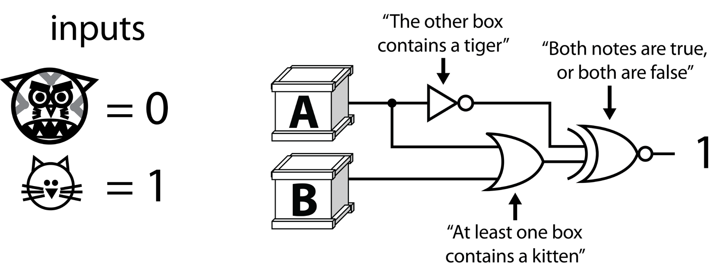
Figure 10-7. A digital solution to the problem
“I’ve set it up so that 0 means tiger and 1 means kitten”, she proudly declared. “If you input a possibility for what’s in each box, you’ll get a 1 output only if the possibility satisfies all the conditions.”
For each of the three conditions (the notes on the two boxes plus the extra rule her father had added), the princess had included a logic gate in her circuit:
-
For the note on box A, she used an
ORgate, indicating that this constraint would only be satisfied if box A or box B contained a kitten. -
For the note on box B, she used a
NOTgate, indicating that this constraint would only be satisfied if box A did not contain a kitten. -
Finally, for her father’s twist, she added an
XNORgate to the end, which would be satisfied (output true) only if the results of the other two gates were the same as each other, both true or both false.
“That’ll do it. Now I just need to run this on each of the four possible configurations of kittens and tigers to find out which one satisfies all the constraints, and then I’ll know which box to open.”
“Ahem,” said the king.
The princess rolled her eyes, “What now, dad?”
“And… you are only allowed to run your device once.”
“Oh,” said the princess. This presented a real problem. Running the device only once would require her to guess which input configuration to test, and would be unlikely to return a conclusive answer. She’d have a 25% chance of guessing the correct input to try, but if that failed and her circuit produced a 0, she would need to just choose a box randomly and hope for the best. With all of this guessing, and knowing her father, she’d probably get eaten by a tiger. No, conventional digital logic just would not do the job this time.
But fortunately (in a quite circular fashion), the princess had recently read an O’Reilly book on quantum computation. So, gurgling with delight, she once again dashed to her workshop. A few hours later she returned, having built a new, somewhat larger, device. She switched it on, logged in via a secure terminal, ran her program, and cheered in triumph. Running to the correct box, she threw it open and happily hugged her kitten.
The end.
Example 10-2 is the QPU program that the princess used, as illustrated in Figure 10-8. The figure also shows the conventional logic gate that each part of the QPU circuit ultimately implements in phase logic. Let’s check that it works!

Figure 10-8. Logic puzzle: Kitten or tiger?
After just a single run of the QPU program in Example 10-2, we can solve the riddle! Just as in Example 10-1, we use magnitude logic until the final operation, for which we employ phase logic. The circuit output shows clearly (and with 100% probability) that the birthday girl should open box B if she wants a kitten. Our phase-logic subroutines take the place of flip in an AA iteration, so we follow them with the mirror subroutine originally defined in Example 6-1.
As discussed in Chapter 6, the number of times that we need to apply a full AA iteration will depend on the number of qubits involved. Luckily, this time we only needed one! We were also lucky that there was a solution to the riddle (i.e., that some set of inputs did satisfy the boolean statement). We’ll see shortly what would happen if there wasn’t a solution.
Note
Remember the subtlety that the mirror subroutine increases the magnitude of values that have their phases flipped with respect to other ones. This doesn’t necessarily mean that the phase has to be negative for this particular state and positive for the rest, so long as it is flipped with respect to the others. In this case, one of the options will be correct (and have a positive phase) and the others will be incorrect (with a negative phase). But the algorithm works just as well!
General Recipe for Solving Boolean Satisfiability Problems
The princess’s puzzle was, of course, a feline form of a boolean satisfiability problem. The approach that we used to solve the riddle generalizes nicely to other boolean satisfiability problems with a QPU:
-
Transform the boolean statement from the satisfiability problem in question into a form having a number of clauses that have to be satisfied simultaneously (i.e., so that the statement is the
ANDof a number of independent clauses).7 -
Represent each individual clause using magnitude logic. Doing so will require a number of scratch qubits. As a rule of thumb, since most qubits will be involved in more than one clause, it’s useful to have one scratch qubit per logical clause.
-
Initialize the full QPU register (containing qubits representing all input variables to the statement) in a uniform superposition (using
HADs), and initialize all scratch registers in the ∣0⟩ state. -
Use the magnitude-logic recipes given in Figure 5-25 to build the logic gates in each clause one by one, storing the output value of each logical clause in a scratch qubit.
-
Once all the clauses have been implemented, perform a phase-logic
ANDbetween all the scratch qubits to combine the different clauses. -
Uncompute all of the magnitude-logic operations, returning the scratch qubits to their initial states.
-
Run a
mirrorsubroutine on the QPU register encoding our input variables. -
Repeat the preceding steps as many times as is necessary according to the amplitude amplification formula given in Equation 6-2.
-
Read the final (amplitude-amplified) result by reading out the QPU register.
In the following sections we give two examples of applying this recipe, the second of which illustrates how the procedure works in cases where a statement we’re trying to satisfy cannot actually be satisfied (i.e., no input combinations can yield a 1 output).
Hands-on: A Satisfiable 3-SAT Problem
Consider the following 3-SAT problem:
(a OR b) AND (NOT a OR c) AND (NOT b OR NOT c) AND (a OR c)
Our goal is to find whether any combination of boolean inputs a, b, c can produce a 1 output from this statement. Luckily, the statement is already the AND of a number of clauses (how convenient!). So let’s follow our steps. We’ll use a QPU register of seven qubits—three to represent our variables a, b, and c, and four scratch qubits to represent each of the logical clauses. We then proceed to implement each logical clause in magnitude logic, writing the output from each clause into the scratch qubits. Having done this, we implement a phase-logic AND statement between the scratch qubits, and then uncompute each of the magnitude-logic clauses. Finally, we apply a mirror subroutine to the seven-qubit QPU register, completing our first amplitude amplification iteration. We can implement this solution with the sample code in Example 10-3, as shown in Figure 10-9.

Figure 10-9. A satisfiable 3-SAT problem
Using circle notation to follow the progress of the three qubits representing a, b, and c, we see the results shown in Figure 10-10.

Figure 10-10. Circle notation for a satisfiable 3-SAT problem after one iteration
This tells us that the boolean statement can be satisfied by values a=1, b=0, and c=1.
In this example, we were able to find a set of input values that satisfied the boolean statement. What happens when no solution exists? Luckily for us, NP problems like boolean satisfiability are such that although finding an answer is computationally expensive, checking whether an answer is correct is computationally cheap. If a problem is unsatisfiable, no phase in the register will get flipped and no magnitude will change as a consequence of the mirror operation. Since we start with an equal superposition of all values, the final READ will give one value from the register at random. We simply need to check whether it satisfies the logical statement; if it doesn’t, we can be sure that the statement is unsatisfiable. We’ll consider this case next.
Hands-on: An Unsatisfiable 3-SAT Problem
Now let’s look at an unsatisfiable 3-SAT problem:
(a OR b) AND (NOT a OR c) AND (NOT b OR NOT c) AND (a OR c) AND b
Knowing that this is unsatisfiable, we expect that no value assignment to variables a, b, and c will be able to produce an output of 1. Let’s determine this by running the QPU routine in Example 10-4, as shown in Figure 10-11, following the same prescription as in the previous example.

Figure 10-11. An unsatisfiable 3-SAT problem
So far, so good! Figure 10-12 shows how the three qubits encoding the a, b, and c input values are transformed throughout the computation. Note that we only consider a single AA iteration, since (as we can see in the figure) its effect, or lack thereof, is clear after only one iteration.

Figure 10-12. Circle notation for an unsatisfiable 3-SAT problem
Nothing has happened! Since none of the eight possible values of the register satisfy the logical statement, no phase has been flipped with respect to any others; hence, the mirror part of the amplitude amplification iteration has equally affected all values. No matter how many AA iterations we perform, when READing these three qubits we will obtain one of the eight values completely at random.
The fact that we could equally have obtained any value on READing might make it seem like we learned nothing, but whichever of these three values for a, b, and c we READ, we can try inputting them into our boolean statement. If we obtain a 0 outcome then we can conclude (with high probability) that the logical statement is not satisfiable (otherwise we would have expected to read out the satisfying values).
Speeding Up Conventional Algorithms
One of the most notable features of amplitude amplification is that, in certain cases, it can provide a quadratic speedup not only over brute-force conventional algorithms, but also over the best conventional implementations.
The algorithms that amplitude amplification can speed up are those with one-sided error. These are algorithms for decision problems containing a subroutine outputting a yes/no answer, such that if the answer to the problem is “no,” the algorithm always outputs “no,” while if the answer to the problem is “yes,” the algorithm outputs the answer “yes” with probability p > 0. In the case of 3-SAT, which we have seen in the previous examples, the algorithms outputs the the “yes” answer (the formula is satisfiable) only if it finds a satisfiable assignment.
To find a solution with some desired probability, these conventional algorithms must repeat their probabilistic subroutine some number of times (k times if the algorithm has a runtime of O). To obtain a QPU speedup, combine them with the quantum routine we simply need to substitute the repeated probabilistic subroutine with an amplitude amplification step.
Any conventional algorithm of this form can be combined with amplitude amplification to make it faster. For example, the naive approach to solving 3-SAT in the earlier examples runs in O(1.4, while the best conventional algorithm runs faster, in O(1.3. However, by combining this conventional result with amplitude amplification, we can achieve a runtime of O(1.1!
There are a number of other algorithms that can be sped up using this technique. For example:
- Element distinctness
-
Algorithms which, given a function f acting on a register, can determine whether there exist two distinct elements in the register i, j for which f(i) = f(j). This problem has applications such as finding triangles in graphs or calculating matrix products.
- Finding global minima
-
Algorithms which, given an integer-valued function acting on a register with N entries, find the index i of the register such that f(i) has the lowest value.
Chapter 14 provides a reference list where many of these algorithms can be found.
1 In the literature, a function that flips phases according to some logic function is referred to as an oracle, in a similar sense to how the term is used in conventional computer science. We opt for slightly less intimidating terminology here, but more thoroughly relate this to prevalent technical language in Chapter 14.
2 We provide a more detailed description of this class of problems at the end of this chapter and in Chapter 14.
3 For example, the phase-logic XOR in Figure 10-2 uses a scratch qubit, which is prepared in the ∣–⟩ state using a NOT and a HAD operation.
4 Note that there are some redundant operations in this circuit (e.g., canceling NOT operations). We have kept these for clarity.
5 Boolean satisfiability was the first problem proven to be NP-complete. N-SAT, the boolean satisfiability problem for boolean statements containing clauses of N literals, is NP-complete when N > 2. In Chapter 14 we give more information about basic computational complexity classes, as well as references to more in-depth material.
6 Adaptation of a logic puzzle from the book The Lady or the Tiger? by Raymond Smullyan.
7 This form is the most desirable, since the final pAND combining all the statements in phase logic can be implemented using a single CPHASE with no need for extra scratch qubits. However, other forms can be implemented with carefully prepared scratch qubits.