CHAPTER
14

Confidence Intervals

In This Chapter

• Interpreting the meaning of a confidence interval
• Calculating the confidence interval for the mean when the population standard deviation is known and when it is unknown
• Introducing the Student’s t-distribution
• Calculating the confidence interval for the proportion
• Determining sample sizes to attain a specific margin of error

Now that we have learned how to collect a random sample and how sample means and sample proportions behave under certain conditions, we are ready to put those samples to work using confidence intervals.

One of the most important roles that statistics plays in today’s world is to gather information from a sample and use that information to make a statement about the population from which it was chosen. We are using the sample as an estimate for the population. But just how good of an estimate is the sample providing us? The concept of confidence intervals will provide us with that answer.

Since we are using the sample statistic (such as the sample mean) as an estimate for the population parameter, we need to distinguish between the point estimate and the interval estimate. Read on.

Point Estimate and Interval Estimate

The simplest estimate of a population is the point estimate, the most common being the sample mean and the sample proportion. A point estimate is a single value that best describes the population of interest. Let me explain this concept by using the following example. Let’s say I’m interested in knowing the average number of carbohydrates in a bowl of cereal. So I collected a random sample of 30 different cereals and found that the average is 29 grams of carbohydrates. I could use that as my point estimate for the number of carbohydrates in the population of all cereals.

The advantage of a point estimate is that it is easy to calculate and easy to understand. The disadvantage, however, is that I have no clue as to how representative of the population it really is.

To deal with this uncertainty, we can use an interval estimate, which provides a range of values within which the population parameter may lie. Confidence intervals provide us with a confidence level that the population parameter is within the interval.

The Principle of Confidence Intervals

Let’s start with the confidence interval for the population mean using a large sample size, which generally refers to n ≥ 30. The large sample enables us to use the Central Limit Theorem (yes, it comes back!). The Central Limit Theorem assures us that with our large sample, the sample mean will be normally distributed regardless of the population distribution.

To develop a confidence interval estimate, we need to learn about confidence levels. A confidence level is the probability that the interval estimate will include the population parameter. The common levels used by statisticians are 90 percent, 95 percent, and 99 percent. In our cereal example, let’s say the 95 percent confidence interval is 25.87 to 32.13 grams of carbohydrates. (We will see in the next section how to get this interval.) This means that I’m 95 percent confident that the average number of grams of carbohydrates in all cereals is between 25.87 and 32.13.

The Probability of an Error (the Alpha Value)

For the 95 percent confidence interval, 95 percent of all intervals will contain the population mean. The other 5 percent of the intervals won’t contain the population mean. This is called the alpha (α) value, the level of significance, or the probability of making a Type I error. (Yes, there is Type II error.) We can write α as

α = 1 – confidence level

For example, the significance level for a 90 percent confidence interval is 10 percent, the significance level for a 99 percent confidence interval is 1 percent, and so on. In general, a (1 – α) confidence interval has a significance level equal to α.

We will revisit the level of significance in more detail in later chapters.

When the Population Standard Deviation Is Known

Since the sample means follow the normal probability distribution because of the central limit theorem, we can use the standard normal distribution table to get the value for z that corresponds to our confidence level. How do we do that? Let’s go back to our cereal carbohydrate example. I want to find a 95 percent confidence interval for the population mean, which is the average number of grams of carbohydrates in all cereals. So far, we know that the sample of 30 cereals has a mean of 29 grams, but I still need two more pieces of information: the population standard deviation (σ) and the z-value corresponding to the 95 percent confidence level. Let’s say σ is 8.74 grams. Now how do we get the z-value?

As Figure 14.1 shows, the shaded area represents the 95 percent confidence level we chose. The un-shaded areas represent the α value, which is 0.05. Since the un-shaded area is divided into two equal areas (because the normal distribution is symmetrical around the mean), each tail represents 0.05/2 = 0.025. To get the value of z, look at the standard normal table in Appendix B and search inside the body of the table for the closest number to 0.0250. (Hint: Look at the negative z-value side because right now we are to the left of the mean.) You will find 0.0250 in the -1.9 row and 0.06 column. So our z-value to the left of the mean is -1.96. Since the distribution is symmetrical, I know you just want to use the same value, but positive, for the right side of the mean. Good idea! Your z-value is +1.96 for the right tail. Now, I can tell you understand the normal distribution pretty well!

Since we will be using these z-values a lot, it might be a good idea to keep them handy. I’ll list the common ones for you:

99% confidence level, z = ±2.58

95% confidence level, z = ±1.96

90% confidence level, z = ±1.65

Figure 14.1

A 95 percent confidence interval.

Now we are ready to find the confidence interval. We can construct a confidence interval around our sample mean using the following equation:

The upper limit of the confidence interval is:

The lower limit of the confidence interval is:

where:

= the sample mean

z_α/2 = the critical z-value, which is the number of standard deviations based on the confidence level

= the standard error of the mean (remember our friend from Chapter 13?)

The term is referred to as the margin of error, or ME, a phrase often referred to in polls and surveys.

Going back to our cereal carbohydrate example, the average number of grams of carbohydrates in our sample of 30 is 29 grams, and the population standard deviation is 8.74 grams. (This represents the variation among different cereals in the population.) We can calculate our 95 percent confidence interval as follows:

= 29 grams, n = 30, σ = 8.74 grams, and Z_α/2 = ±1.96

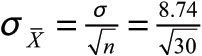=1.5957

Upper limit = =29 + 1.96(1.5957) = 32.13

Lower limit = = 29 – 1.96(1.5957) = 25.87

According to this result, our 95 percent confidence interval for this random sample of cereal carbohydrates is between 25.87 and 32.13 grams. In other words, we are 95 percent confident that the number of grams of carbohydrates for all cereals is between 25.87 and 32.13 (or 25.87, 32.13).

Another way to get this interval is by using the margin of error. The margin of error (ME) = . So in our example, ME = (1.96)(1.5957) = 3.13. The 95 percent confidence interval is = 29 ± 3.13 = (25.87, 32.13). As you can see from this example, finding the 95 percent confidence interval this way is very simple. We start with the sample mean, then we add the margin of error to get the upper limit of the interval and subtract the margin of error to get the lower limit of the interval. Easy, isn’t it? This interval is shown in Figure 14.2.

Figure 14.2

A 95 percent confidence interval for cereal’s average number of grams of carbohydrates.

Figure 14.3

Interpreting the definition of a confidence interval.

Because there is a 95 percent probability that any given confidence interval will contain the true population mean in the previous example, we have a 5 percent chance that it won’t. This 5 percent value is the level of significance, α, which is represented by the total white area in both tails of Figure 14.3.

The Effect of Changing Confidence Levels

So far, we have only referred to a 95 percent confidence interval. However, we can choose other confidence levels to suit our needs. The following table shows our cereal carbohydrate example with confidence levels of 90, 95, and 99 percent.

Confidence Intervals with Various Confidence Levels

From the previous table, you can see that there’s a price to pay for increasing the confidence level–our interval estimate of the true population mean becomes wider. We have proven that, once again, there is no free lunch with statistics. If you want more certainty that your confidence interval will contain the true population mean, then your confidence interval will become wider.

I’ve a feeling that you notice something else: as the confidence level increases, so does the margin of error. Yes, that’s why the interval gets wider.

The Effect of Changing the Sample Size

There is one way, however, to reduce the width of our confidence interval while maintaining the same confidence level. We can do this by increasing the sample size. There is still no free lunch though because increasing the sample size has a cost associated with it. Let’s say we increase our sample size to include 62 different cereals. This change will affect our standard error as follows:

= 1.11 grams

Our new 95 percent confidence interval for our original sample will be:

= 29 grams, n = 62, grams = 1.11 grams

Upper limit = = 29 + 1.96(1.11) = 31.18 grams

Lower limit = = 29 – 1.96(1.11) = 26.82 grams

Increasing our sample size from 30 to 62 has reduced the 95 percent confidence interval from (25.87, 32.13) to (26.82, 31.18). Can you tell what will happen to the margin of error when I increase my sample size? It will also decrease. As n increases to 62, the margin of error is now = 1.96(1.11) = 2.18 grams, compared with 3.13 grams when n = 30.

So far we have seen how to get the confidence interval for the population mean when sigma is known and we have a large sample (n ≥ 30). What if we have a small sample instead? The bad news, in this case, is we can’t use the central limit theorem, so the population from which the sample is drawn must be normally distributed. The good news is, if the population is normally distributed, then we can construct the confidence interval for a small sample the same way as we did with the large sample.

When the Population Standard Deviation Is Unknown

Here’s a simple section for you. (It’s about time!) So far we have assumed that we know σ, the population standard deviation. What happens if σ is unknown? Don’t panic, we can substitute s, the sample standard deviation, for σ, the population standard deviation, and then follow the same procedure as before as long as we have a large sample. In this case, the confidence interval will be where . Let’s see an example to illustrate this large sample case, and then we’ll move to the small sample instance.

Consider the following table that shows the number of grams of carbohydrates in a sample of 32 different cereals.

Cereal Carbohydrate Grams Sample (n = 32)

Using Excel, we can confirm that:

= 30 grams and s = 8.97 grams

A 99 percent confidence interval around this sample mean would be:

Upper limit = grams

Lower limit = grams

We can also use the margin of error approach here. In this example, ME = 2.58(1.59) = 4.10. When you subtract this from 30, you get the lower limit as 25.9 grams, and when you add it to 30, you get the upper limit of the interval as 34.1 grams.

See! That wasn’t too bad.

When the Population Standard Deviation Is Unknown and with Small Samples

When σ is unknown and we have a small sample, we can’t use the standard normal distribution anymore. This substitution forces us to use a new probability distribution known as the Student’s t-distribution (named in honor of you, the student).

The t-distribution is a continuous probability distribution with the following properties:

• It is bell-shaped and symmetrical around the mean.
• The shape of the curve depends on the degrees of freedom (d.f.) which, when dealing with the sample mean, would be equal to n – 1.
• The area under the curve is equal to 1.0.
• The t-distribution has a mean of zero, just like the normal distribution, but a variance greater than one.
• The t-distribution is flatter than the normal distribution. As the number of degrees of freedom increases, the shape of the t-distribution becomes similar to the normal distribution as seen in Figure 14.4. With more than 30 degrees of freedom (a sample size of 30 or more), the two distributions are practically identical.

Figure 14.4

The Student’s t-distribution compared to the normal distribution.

Students often struggle with the concept of degrees of freedom, which represent the number of remaining free choices you have after something has been decided, such as the sample mean. For example, if I know that my sample of size 3 has a mean of 10, I can only vary two values (n – 1). After I set those two values, I have no control over the third value because my sample average must be 10. For this sample, I have 2 degrees of freedom.

We can now set up our confidence intervals for the mean using a small sample:

The upper limit of the confidence interval is

The lower limit of the confidence interval is

where:

t_α/2 = critical t-value (can be found in Table 4 in Appendix B)

= the estimated standard error of the mean

To demonstrate this procedure, let’s assume the population of cereals’ grams of carbohydrates follows a normal distribution and the following sample of 10 cereals were collected.

Number of Grams of Carbohydrates in a Cereal Sample from a Normal Distribution (n = 10)

With σ unknown, we will construct a 95 percent confidence interval around the sample mean as follows:

To determine the value of t_α/2 for this example, I need to calculate the number of degrees of freedom. Because n = 10, I have n – 1 = 9 d.f. This corresponds to t_α/2 = 2.262, which is underlined in the following table taken from Table 4 in Appendix B.

Excerpt from the Student’s t-Distribution:

Selected right-tail areas with confidence levels underneath

We next need to calculate the sample mean and sample standard deviation, which, according to Excel, are as follows:

= 27 grams and s = 10.83 grams

We can calculate the standard error of the mean:

= 3.42

and can construct our 95 percent confidence interval:

Upper limit = = 34.74 grams

Lower limit = = 19.26 grams

We can still use the margin of error approach as before. In this example, the margin of error is 7.74 grams. I’ll leave it to you to confirm the confidence interval.

Now that wasn’t too bad!

Determining Sample Size for the Population Mean

Knowing the appropriate sample size needed for a specific confidence level and margin of error is very important, especially for quality control. For example, M&M’s bags weigh 1.69 ounces. The producers of M&M’s want to make sure that the bags weigh 1.69 ounces. Weighing every single M&M’s bag is costly and time consuming, so M&M’s producers want to use a sample of M&M’s, weigh them, and check if the weight is 1.69 ounces or not. How large should the sample be? This is what this section is all about.

We can calculate a minimum sample size that would be needed to provide a specific margin of error. In our cereal carbohydrates example, what sample size would we need for a 95 percent confidence interval that has a margin of error of ±3 grams?

Therefore, to obtain a 95 percent confidence interval that ranges from 29 – 3 = 26 grams to 29 + 3 = 32 grams would require a sample size of 33 cereals.

If you want to reduce your margin of error to ±2 grams, you will need a larger sample of ≈74 cereals! Remember, there is no free lunch in statistics!

Using Excel’s CONFIDENCE Function

Excel has a pretty cool built-in function that calculates confidence intervals for us. If you are using the normal distribution, then use the CONFIDENCE.NORM function, and if you are using the t-distribution, then use the CONFIDENCE.T function. The CONFIDENCE.NORM function has the following characteristics:

CONFIDENCE.NORM(alpha, standard_dev, size)

where:

alpha = the significance level of the confidence interval

standard_dev = the standard deviation of the population

size = sample size

For instance, Figure 14.5 shows the CONFIDENCE.NORM function being used to calculate the confidence interval for our original cereal carbohydrates example.

Figure 14.5

CONFIDENCE.NORM function in Excel for the cereal carbohydrates example.

Cell A1 contains the Excel formula =CONFIDENCE.NORM(0.05,8.74,30) with the result being 3.127511. This value represents the margin of error, or the amount to add and subtract from the sample mean, as follows:

29 + 3.13 = 32.13 grams

29 – 3.13 = 25.87 grams

This confidence interval is slightly different from the one calculated earlier in the chapter due to the rounding of numbers.

Now, let’s use Excel to calculate the confidence interval using the t-distribution. The CONFIDENCE.T function has the following characteristics:

CONFIDENCE.T(alpha, standard_dev, size)

where:

alpha = the significance level of the confidence interval

standard_dev = the standard deviation of the sample

size = sample size

For instance, Figure 14.6 shows the CONFIDENCE.T function being used to calculate the confidence interval for our cereal carbohydrates example with a small sample and σ unknown.

Figure 14.6

CONFIDENCE.T function in Excel for the cereal carbohydrates example.

Cell A1 contains the Excel formula =CONFIDENCE.T(0.05,10.83,10) with the result being 7.747315. As with CONFIDENCE.NORM, this value represents the margin of error, or the amount to add and subtract from the sample mean, as follows:

27 + 7.75 = 34.75 grams

27 – 7.75 = 19.25 grams

This confidence interval is also slightly different from the one calculated earlier in the chapter due to the rounding of numbers. This sure beats using tables and square root functions on the calculator.

That ends our discussion on confidence intervals around the mean. Next on the menu is proportions!

Confidence Intervals for the Population Proportion with Large Samples

We can also estimate the proportion of a population by constructing a confidence interval from a sample. As you might recall from Chapter 13, proportion data follow the binomial distribution that can be approximated by the normal distribution under the following conditions:

np ≥ 5 and nq ≥ 5

where:

p = the probability of a success in the population

q = the probability of a failure in the population (q = 1 – p)

Suppose I want to estimate the proportion of high school graduates who enroll in colleges or universities based on the results of a sample. In Chapter 13, we learned that we can calculate the proportion of a sample using:

There’s extra credit for anyone who can see a problem arising here. Our challenge is that we are trying to estimate p, the population proportion, but we need a value for p to set up the confidence interval. Our solution–estimate the standard error by using the sample proportion, , as an approximation for the population proportion as follows:

We now can construct a confidence interval around the sample proportion by:

(upper limit of the confidence interval)

(lower limit of the confidence interval)

Let’s put these equations to work. In my efforts to estimate the proportion of high school graduates who enroll in colleges or universities, I sample 175 random high school graduates, of whom 110 enrolled in colleges or universities. I can now calculate , the sample proportion:

The estimated standard error of the proportion would be:

We are now ready to construct a 95 percent confidence interval around our sample proportion (z_α/2 = 1.96):

Upper limit = + 1.96 = 0.629 + 1.96(0.0365) = 0.70

Lower limit = – 1.96 = 0.629 – 1.96(0.0365) = 0.557

Our 95 percent confidence interval for the proportion of high school graduates who enroll in colleges or universities is (0.56, 0.70), so we are 95 percent confident that between 56 percent and 70 percent of high school graduates enroll in colleges and universities. A reality check, according to the Bureau of Labor Statistics: 68.4 percent of high school graduates enrolled in colleges and universities in 2014. That’s well within our interval!

You can also use the margin of error approach to get the confidence interval for the proportion. In our example, the margin of error is 1.96(0.0365) = 0.0715. Subtracting it and adding it to the mean yields the same confidence interval as before. This is especially useful for the polls we hear in the news. For example, according to Gallup, President Obama’s approval rating on November 5-7, 2015 was 48 percent with a margin of error of ±3 percentage points. This means that the 95 percent confidence interval for President Obama’s approval rating is 45 percent to 51 percent. See, now you understand the small print better!

Determining Sample Size for the Proportion

Just as we did for the mean, we can determine a required sample size that would be needed to provide a specific margin of error. What sample size would we need for a 99 percent confidence interval that has a margin of error of ±6 percent (ME = 0.06) in our example of high school graduates enrolling in college and universities? The formula to calculate n, the sample size is:

Notice that we need a value for here. We have a couple of options:

• If we have a preliminary estimate of from a previous study, we can use it.
• If we don’t have a preliminary estimate, then set p = q = 0.50.

Applying this to our example,

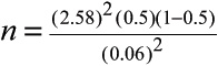= 462.25 ≈ 463

Therefore, to obtain a 99 percent confidence interval that provides a margin of error no more than ±6 percent would require a sample size of 463 high school graduates.

Practice Problems

1. Construct a 97 percent confidence interval around a sample mean of 31.3 taken from a population that is not normally distributed with a standard deviation of 7.6 using a sample of size 40.

2. What sample size would be necessary to ensure a margin of error of 5 for a 98 percent confidence interval taken from a population that is not normally distributed and which has a population standard deviation of 15?

3. Construct a 90 percent confidence interval around a sample mean of 16.3 taken from a population that is not normally distributed with a population standard deviation of 1.8 using a sample of size 10.

4. The following sample of size 30 was taken from a population that is not normally distributed:

10        4        9        12        5        17        20        9        4        15

11        12        16        22        10        25        21        14        9        8

14        16        20        18        8        10        28        19        16        15

 Construct a 90 percent confidence interval around the mean.

5. The following sample of size 12 was taken from a population that is normally distributed and that has a population standard deviation of 12.7:

37        48        30        55        50        46        40        62        50        43        36        66

 Construct a 94 percent confidence interval around the mean.

6. The following sample of size 11 was taken from a population that is normally distributed:

121        136        102        115        126        106        115        132        125        108        130

 Construct a 98 percent confidence interval around the mean.

7. The following sample of size 11 was taken from a population that is not normally distributed:

87        59        77        65        98        90        84        56        75        96        66

 Construct a 99 percent confidence interval around the mean.

8. A sample of 200 light bulbs was tested, and it was found that 11 were defective. Calculate a 95 percent confidence interval around this sample proportion.

9. What sample size would you need to construct a 96 percent confidence interval around the proportion for voter turnout during the next election that would provide a margin of error of 4 percent? Assume the population proportion has been estimated at 55 percent.