
The Binomial Probability Distribution
In This Chapter
![]()
- Describe the characteristics of a binomial experiment
- Calculate the probabilities for a binomial distribution
- Find probabilities using a binomial table
- Find binomial probabilities using Excel
- Calculate the mean and standard deviation of a binomial distribution
Our discussion of discrete probability distributions so far has been limited to general distributions based on historical data that has been previously collected. However, some theoretical probability distributions are based on a mathematical formula rather than historical data. We will address the first of these, the binomial probability distribution, in this chapter.
In many types of problems we are interested in the probability of an event occurring several times. A classical example that has been torturing students for many years is “What is the chance of getting 7 heads when tossing a coin 10 times?” By the time you finish this chapter, answering this question will be a piece of cake!
Characteristics of a Binomial Experiment
If you remember, in Chapter 6 we defined experimenting as the process of measuring or observing an activity for the purpose of collecting data. Let’s say our experiment of interest involves a certain professional basketball player shooting free throws. Each free throw would be considered a trial for the experiment. For this particular experiment, we have only two possible outcomes for each trial; either the free throw goes into the basket (a success) or it doesn’t (a failure). Because we can have only two possible outcomes for each trial, this is known as a binomial experiment.
DEFINITION
A binomial experiment has the following characteristics: (1) the experiment consists of a fixed number of trials denoted by n; (2) each trial has only two possible outcomes, a success or a failure; (3) the probability of success and the probability of failure are constant throughout the experiment; (4) each trial is independent of any other trial in the experiment.
Let’s say that our player of interest is Michael Jordan, who historically has made 80 percent of his free throws. So the probability of success, p, of any given free throw is 0.80. Because there are only two outcomes possible, the probability of failure for any given free throw, q, is 0.20. For a binomial experiment, the values of p and q must be the same for every trial in the experiment. Because only two outcomes are allowed in a binomial experiment, p = 1 – q always holds true.
BOB’S BASICS
The outcomes in the binomial distribution are classified as either success or failure. The word success doesn’t necessarily mean a positive outcome. It is the outcome we are interested in. Likewise, the word failure doesn’t necessarily mean a negative outcome.
Finally, a binomial experiment requires that each trial is independent of any other trial. In other words, the probability of the second free throw being successful is not affected by whether the first free throw was successful. Other examples of binomial experiments include the following:
- Testing whether a part is defective after it has been manufactured
- Observing the number of correct responses in a multiple-choice exam
- Counting the number of American households that have an internet connection
Now that we have defined the ground rules for binomial experiments, we are ready to graduate to calculating binomial probabilities.
The Binomial Probability Distribution
The binomial probability distribution allows us to calculate the probability of a specific number of successes for a certain number of trials. Therefore, the random variable for this distribution would be the number of successes that were observed. To demonstrate a binomial distribution, I will use the following example.
Suppose that the probability of passing an exam is 60 percent, so the probability of failing the exam is 40 percent. This represents a binominal experiment, with p = 0.60 (the probability of a “success”) and q = 0.40 (the probability of a “failure”). We can calculate the probability of x successes in n trials using the binomial distribution, as follows:
![]()
Where:
n: the total number of trials
x: the number of successes
p: the probability of a success
q: the probability of failure
P(x): the probability of observing x number of successes in n number of trials.
If the class has five students, with this equation, we can calculate the probability that three students will pass the exam as follows:
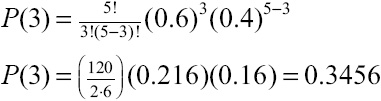
There is a 34.56 percent chance that three students out of the class of five students will pass the exam. We can also calculate the probability that zero, one, two, four, or five students will pass the exam as follows:
BOB’S BASICS
Remember from Chapter 7, 0! = 1. Also x0 = 1 for any value of x.
For x = 0:


For x = 2:

For x = 4:

For x = 5:

The following table summarizes all the previous probabilities.
x |
P(x) |
0 |
0.0102 |
1 |
0.0768 |
2 |
0.2304 |
3 |
0.3456 |
4 |
0.2595 |
5 |
0.0778 |
Total = 1.0 |
This table represents the binomial probability distribution for x successes in five trials with the probability of success equal to 0.60. Notice that the sum of all the probabilities equals 1, which is a requirement for all probability distributions. Figure 9.1 shows this probability distribution as a histogram.

Figure 9.1
Binomial probability distribution.
From this figure, we can see that the most likely number of students who will pass the exam out of the class of 5 students is 3.
Finally, we can calculate the probability of multiple events for this distribution. For instance, the probability that three or more students in the class will pass the exam is this:

Also, the probability that one or less students in the class will pass the exam is:

This looks like a good class!
Binomial Probability Tables
As the number of trials increases in a binomial experiment, calculating probabilities using the previous formula will really drain the batteries in your calculator and possibly even your brain. An easier way to arrive at these probabilities is to use a binomial probability table, which I have conveniently provided in Appendix B of this book. Following is an excerpt from this appendix, with the probabilities from our previous example underlined.
The probability table is organized by values of n, the total number of trials. The number of successes, x, are the rows of each section, whereas the probability of success, p, are the columns. Notice that the sum of each block of probabilities for a particular value of p adds to 1.0.
Values of p

One limitation of using binomial tables is that you are restricted to using only the values of p that are shown in the table. For instance, the previous table would not be useful for p = 0.35. Other statistics books may contain binomial tables that are more extensive than the one in Appendix B.
Using Excel to Calculate Binomial Probabilities
A convenient way to calculate binomial probabilities is to rely on our friend Excel, with its BINOM.DIST function. This built-in function has the following characteristics:
BINOM.DIST(x, n, p, cumulative)
where:
cumulative = FALSE if you want the probability of exactly x successes
cumulative = TRUE if you want the probability of x or fewer successes
For instance, Figure 9.2 shows the BINOM.DIST function being used to calculate the probability that two students out of the class of five will pass the exam.

Figure 9.2
BINOM.DIST function in Excel for exactly x successes.
Cell A1 contains the Excel formula =BINOM.DIST(2,5,0.6,FALSE) with the result being 0.2304.
Excel will also calculate the probability that no more than two students out of the class of five will pass the exam, as shown in Figure 9.3.

Figure 9.3
BINOM.DIST function in Excel for no more than x successes.
Cell A6 contains the Excel formula =BINOM.DIST(2,5,0.6,TRUE) with the result being 0.31744, which is the same as this:

In other words, there is about 32 percent chance that no more than two students out of the class of 5 will pass the exam.
One benefit of using Excel to determine binomial probabilities is that you are not limited to the values of p shown in the binomial table in Appendix B. Excel’s BINOM.DIST function allows you to use any value between 0 and 1 for p.
The Mean and Standard Deviation for the Binomial Distribution
You can calculate the mean for a binomial probability distribution by using the following equation:
![]()
where:
n = the number of trials
p = the probability of a success
For our example, the mean of the distribution is as follows:
![]()
In other words, on average, 3 out of the class of five students will pass the exam.
You can calculate the standard deviation for a binomial probability distribution using the following equation:
![]()
where:
q = the probability of a failure
For our example, the standard deviation of the distribution is as follows:
![]()
Well, that about covers the binomial probability distribution discussion. Don’t be too sad, though; you’ll see this again in future chapters.
Practice Problems
1. What is the probability of seeing exactly 7 heads after tossing a coin 10 times?
2. Goldey-Beacom College accepts 75 percent of applications that are submitted for entrance. What is the probability that they will accept exactly three of the next six applications?
3. Michael Jordan makes 80 percent of his free throws. What is the probability that he will make at least six of his next eight free-throw attempts?
4. A student randomly guesses at a 12-question, multiple-choice test where each question has 5 choices. What is the probability that the student will correctly answer exactly six questions?
5. Historical records show that 5 percent of people who visit a particular website purchase something. What is the probability that no more than two people out of the next seven will purchase something?
6. During the 2005 Major League Baseball season, Derrek Lee had a 0.335 batting average. Construct a binomial probability distribution for the number of successes (hits) for four official at bats during this season.
7. Sixty percent of a particular college population are female students. What is the probability that a class of 10 students has exactly 4 female students?
The Least You Need to Know
- A binomial experiment has only two possible outcomes for each trial.
- For a binomial experiment, the probability of success and failure is constant.
- Each trial of a binomial experiment is independent of any other trial in the experiment.
- The probability of x successes in n trials using the binomial distribution is as follows:

- Calculate the mean for a binomial probability distribution by using the equation

- Calculate the standard deviation for a binomial probability distribution by using the equation
