
11.5.4. Storage Methods
Regardless of whether we want to use full precomputed lighting or to precalculate the transfer information and allow for some changes in the lighting, the resulting data has to be stored in some form. GPU-friendly formats are a must.
Light maps are one of the most common way of storing precomputed lighting. These are textures that store the precalculated information. Though sometimes terms such as irradiance map are used to denote a specific type of data stored, the term light maps is used to collectively describe all of these.
At runtime, the GPU’s built-in texture mechanisms are used. Values are usually bilinearly filtered, which for some representations might not be entirely correct. For example, when using an AHD representation, the filtered D (direction) component will no longer be a unit length after interpolation and so needs to be renormalized.
Using interpolation also means that the A (ambient) and H (highlight) are not exactly
what they would be if we computed them directly at the sampling point. That said, the results usually look acceptable, even if the representation is nonlinear.
In most cases light maps do not use mipmapping, which is normally not needed because the resolution of the light map is small compared to typical albedo maps or normal maps. Even in high-quality applications, a single light-map texel covers the area of at least roughly centimeters, often more. With texels of this size, extra mip levels would almost never be needed.

Figure 11.27. Light baked into a scene, along with the light maps applied to the surfaces. Light mapping uses a unique parameterization. The scene is divided into elements that are flattened and packed into a common texture. For example, the section in the lower left corresponds the ground plane, showing the two shadows of the cubes. (From the three.js example webgl_materials_lightmap [218].)
To store lighting in the texture, objects need to provide an unique parameterization. When mapping a diffuse color texture onto a model, it is usually fine for different parts of the mesh to use the same areas of the texture, especially if a model is textured with a general repeating pattern. Reusing light maps is difficult at best. Lighting is unique for every point on the mesh, so every triangle needs to occupy its own, unique area on the light map. The process of creating a parameterization starts with splitting the meshes into smaller chunks. This can be done either automatically, using some heuristics [1036], or by hand, in the authoring tool. Often, the split that is already present for the mapping of other textures is used. Next, each chunk is parameterized independently, ensuring that its parts do not overlap in texture space [1057,1617]. The resulting elements in texture space are called charts or shells. Finally, all the charts are packed into a common texture (Figure 11.27). Care must be taken to ensure that not only do charts not overlap, but also their filtering footprints must stay separate. All the texels that can be accessed when rendering a given chart (bilinear filtering accesses four neighboring texels) should be marked as used, so no other chart overlaps them. Otherwise, bleeding between the charts might occur, and lighting from one of them might be visible on the other. Although it is fairly common for light mapping systems to provide a user-controlled “gutter” amount for spacing between the light map charts, this separation is not necessary. The correct filtering footprint of a chart can be determined automatically by rasterizing it in light-map space, using a special set of rules. See Figure 11.28. If shells rasterized this way do not overlap, we are guaranteed that no bleeding will happen.

Figure 11.28. To accurately determine the filtering footprint of a chart, we need to find all texels that can be accessed during rendering. If a chart intersects a square spanned between the centers of four neighboring texels, all of them will be used during bilinear filtering. The texel grid is marked with solid lines, texel centers with blue dots, and the chart to be rasterized with thick, solid lines (left). We first conservatively rasterize the chart to a grid shifted by half of a texel size, marked with dashed lined (center). Any texel touching a marked cell is considered occupied (right).
Avoiding bleeding is another reason why mipmapping is rarely used for light maps. Chart filtering footprints would need to stay separate on all the mip levels, which would lead to excessively large spacing between shells.
Optimally packing charts into textures is an NP-complete problem, which means that there are no known algorithms that can generate an ideal solution with polynomial complexity. As real-time applications may have hundreds of thousands charts in a single texture, all real-world solutions use fine-tuned heuristics and carefully optimized code to generate packing quickly [183,233,1036]. If the light map is later block-compressed (Section ), to improve the compression quality additional constraints might be added to the packer to ensure that a single block contains only similar values.
A common problem with light maps are seams (Figure 11.29). Because the meshes are split into charts and each of these is parameterized independently, it is impossible to ensure that the lighting along split edges is exactly the same on both sides. This manifests as a visual discontinuity. If the meshes are split manually, this problem can be avoided somewhat by splitting them in areas that are not directly visible. Doing so, however, is a laborious process, and cannot be applied when generating the parameterizations automatically. Iwanicki [806] performs a post-process on the final light map that modifies the texels along the split edges to minimize the difference between the interpolated values on both sides. Liu and Ferguson et al. [1058] enforce interpolated values matching along the edge via an equality constraint and solve for texel values that best preserve smoothness. Another approach is to take this constraint into account when creating parameterization and packing charts. Ray et al. [1467] show how grid-preserving parameterization can be used to create light maps that do not suffer from seam artifacts.
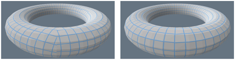
Figure 11.29. To create a unique parameterization for a torus, it needs to be cut and unwrapped. The torus on the left uses a simple mapping, created without considering how the cuts are positioned in texture space. Notice the discontinuities of the grid representing texels on the left. Using more advanced algorithms, we can create a parameterization that ensures that the texel grid lines stay continuous on the three-dimensional mesh, as on the right. Such unwrapping methods are perfect for light mapping, as the resulting lighting does not exhibit any discontinuities.
Precomputed lighting can also be stored at vertices of the meshes. The drawback is that the quality of lighting depends on how finely the mesh is tessellated. Because this decision is usually made at an early stage of authoring, it is hard to ensure that there are enough vertices on the mesh to look good in all expected lighting situations. In addition, tessellation can be expensive. If the mesh is finely tessellated, the lighting signal will be oversampled. If directional methods of storing the lighting are used, the whole representation needs to be interpolated between the vertices by the GPU and passed to the pixel shader stage to perform the lighting calculations. Passing so many parameters between vertex and pixels shaders is fairly uncommon, and generates workloads for which modern GPUs are not optimized, which causes inefficiencies and lower performance. For all these reasons, storing precomputed lighting on vertices is rarely used.
Even though information about the incoming radiance is needed on the surfaces (except when doing volumetric rendering, discussed in Chapter 14), we can precompute and store it volumetrically. Doing so, lighting can be queried at an arbitrary point in space, providing illumination for objects that were not present in the scene during the precomputation phase. Note, however, that these objects will not correctly reflect or occlude lighting.
Greger et al. [594] present the irradiance volume, which represents the five-dimensional (three spatial and two directional) irradiance function with a sparse spatial sampling of irradiance environment maps. That is, there is a three-dimensional grid in space, and at each grid point is an irradiance environment map. Dynamic objects interpolate irradiance values from the closest maps. Greger et al. use a two-level adaptive grid for the spatial sampling, but other volume data structures, such as octrees [1304,1305], can be used.
In the original irradiance volume, Greger et al. stored irradiance at each sample point in a small texture, but this representation cannot be filtered efficiently on the GPU. Today, volumetric lighting data are most often stored in three-dimensional textures, so sampling the volume can use the GPU’s accelerated filtering. The most common representations for the irradiance function at the sample points include:
- Spherical harmonics (SH) of second- and third-order, with the former being more common, as the four coefficients needed for a single color channel conveniently pack into four channels of typical texture format.
- Spherical Gaussians.
- Ambient cube or ambient dice.
The AHD encoding, even though technically capable of representing spherical irradiance, generates distracting artifacts. If SH is used, spherical harmonic gradients [54] can further improve quality. All of the above representations have been successfully used in many games [766,808,1193,1268,1643].
Evans [444] describes a trick used for the irradiance
volumes in LittleBigPlanet. Instead of a full irradiance map representation, an average irradiance is stored at each point. An approximate directionality factor is computed from the gradient of the irradiance field, i.e., the direction in which the field changes most rapidly. Instead of computing the gradient explicitly, the dot product between the gradient and the surface normal is computed by taking two samples of the irradiance field, one at the surface point and another at a point displaced slightly in the direction of , and subtracting one from the other. This approximate representation is motivated by the fact that the irradiance volumes in LittleBigPlanet are computed dynamically.
Irradiance volumes can also be used to provide lighting for static surfaces. Doing so has the advantage of not having to provide a separate parameterization for the light map. The technique also does not generate seams. Both static and dynamic objects can use the same representation, making lighting consistent between the two types of geometry. Volumetric representations are convenient for use in deferred shading (Section ), where all lighting can be performed in a single pass. The main drawback is memory consumption. The amount of memory used by light maps grows with the square of their resolution; for a regular volumetric structure it grows with the cube. For this reason, considerably lower resolutions are used for grid volume representations. Adaptive, hierarchical forms of lighting volumes have better characteristics, but they still store more data than light maps. They are also slower than a grid with regular spacing, as the extra indirections create load dependencies in the shader code, which can result in stalls and slower execution.
Storing surface lighting in volumetric structures is somewhat tricky. Multiple surfaces, sometimes with vastly different lighting characteristics, can occupy the same voxel, making it unclear what data should be stored. When sampling from such voxels, the lighting is frequently incorrect. This happens particularly often near the walls between brightly lit outdoors and dark indoors, and results in either dark patches outside or bright ones inside. The remedy for this is to make the voxel size small enough to never straddle such boundaries, but this is usually impractical because of the amount of data needed. The most common ways of dealing with the problem are shifting the sampling position along the normal by some amount, or tweaking the trilinear blending weights used during interpolation. This is often imperfect and manual tweaks to the geometry to mask the problem might be needed. Hooker [766] adds extra clipping planes to the irradiance volumes, which limit their influence to the inside of a convex polytope. Kontkanen and Laine [926] discuss various strategies to minimize bleeding.
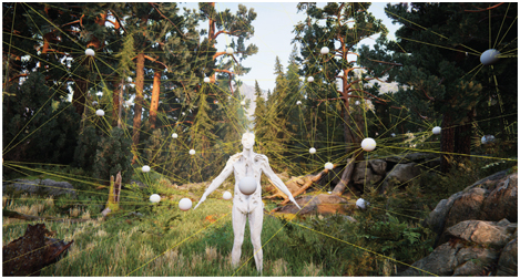
Figure 11.30. Unity engine uses a tetrahedral mesh to interpolate lighting from a set of probes. (Book of the Dead © Unity Technologies, 2018.)
The volumetric structure that holds the lighting does not have to be regular. One popular option is to store it in an irregular cloud of points that are then connected to form a Delaunay tetrahedralization (Figure 11.30). This approach was popularized by Cupisz [316]. To look up the lighting, we first find the tetrahedron the sampling position is in. This is an iterative process and can be somewhat expensive. We traverse the mesh, moving between neighboring cells. Barycentric coordinates of the lookup point with respect to the current tetrahedron corners are used to pick the neighbor to visit in the next step (Figure 11.31). Because typical scenes can contain thousands of positions in which the lighting is stored, this process can potentially be time consuming. To accelerate it, we can record a tetrahedron used for lookup in the previous frame (when possible) or use a simple volumetric data structure that provides a good “starting tetrahedron” for an arbitrary point in the scene.
Once the proper tetrahedron is located, the lighting stored on its corners is interpolated, using the already-available barycentric coordinates. This operation is not accelerated by the GPU, but it requires just four values for interpolation, instead of the eight needed for trilinear interpolation on a grid.

Figure 11.31. Process of a lookup in a tetrahedral mesh illustrated in two dimensions. Steps are shown left to right, top to bottom. Given some starting cell (marked in blue), we evaluate the barycentric coordinates of the lookup point (blue dot) with respect to the cell’s corners. In the next step, we move toward the neighbor across the edge opposite to the corner with the most negative coordinate.
The positions for which the lighting gets precomputed and stored can be placed manually [134,316] or automatically [809,1812]. They are often referred to as lighting probes, or light probes, as they probe (or sample) the lighting signal. The term should not be confused with a “light probe” (Section 10.4.2), which is the distant lighting recorded in an environment map.
The quality of the lighting sampled from a tetrahedral mesh is highly dependent upon the structure of that mesh, not just the overall density of the probes. If they are distributed nonuniformly, the resulting mesh can contain thin, elongated tetrahedrons that generate visual artifacts. If probes are placed by hand, problems can be easily corrected, but it is still a manual process. The structure of the tetrahedrons is not related to the structure of the scene geometry, so if not properly handled, lighting will be interpolated across the walls and generate bleeding artifacts, just as with irradiance volumes. In the case of manual probe placement, users can be required to insert additional probes to stop this from happening. When automated placement of probes is used, some form of visibility information can be added to the probes or tetrahedrons to limit their influence to only relevant areas [809,1184,1812].
It is a common practice to use different lighting storage methods for static and dynamic geometry. For example, static meshes could use light maps, while dynamic objects could get lighting information from volumetric structures. While popular, this scheme can create inconsistencies between the looks of different types of geometry. Some of these differences can be eliminated by regularization, where lighting information is averaged across the representations.
When baking the lighting, care is needed to compute its values only where they are truly valid. Meshes are often imperfect. Some vertices may be placed inside geometry, or parts of the mesh may self-intersect. The results will be incorrect if we compute incident radiance in such flawed locations. They will cause unwanted darkening or bleeding of incorrectly unshadowed lighting. Kontkanen and Laine [926] and Iwanicki and Sloan [809] discuss different heuristics that can be used to discard invalid samples.
Ambient and directional occlusion signals share many of the spatial characteristics of diffuse lighting. As mentioned in Section 11.3.4, all of the above methods can be used for storing them as well.
11.5.5. Dynamic Diffuse Global Illumination
Even though precomputed lighting can produce impressive-looking results, its main strength is also its main weakness—it requires precomputation. Such offline processes can be lengthy. It is not uncommon for lighting bakes to take many hours for typical game levels. Because lighting computations take so long, artists are usually forced to work on multiple levels at the same time, to avoid downtime while waiting for the bakes to finish. This, in turn, often results in an excessive load on the resources used for rendering, and causes the bakes to take even longer. This cycle can severely impact productivity and cause frustration. In some cases, it is not even possible to precompute the lighting, as the geometry changes at runtime or is created to some extent by the user.
Several methods have been developed to simulate global illumination in dynamic environments. Either they do not require any preprocessing, or the preparation stage is fast enough to be executed every frame.
One of the earliest methods of simulating global illumination in fully dynamic environments was based on “Instant Radiosity” [879]. Despite the name, the method has little in common with the radiosity algorithm. In it, rays are cast outward from the light sources. For each location where a ray hits, a light is placed, representing the indirect illumination from that surface element. These sources are called virtual point lights (VPLs). Drawing upon this idea, Tabellion and Lamorlette [1734] developed a method used during production of Shrek 2 that performs a direct lighting pass of scene surfaces and stores the results in textures. Then, during rendering, the method traces rays and uses the cached lighting to create one-bounce indirect illumination. Tabellion and Lamorlette show that, in many cases, a single bounce is enough to create believable results. This was an offline method, but it inspired a method by Dachsbacher and Stamminger [321] called reflective shadow maps (RSM).
Similar to regular shadow maps (Section 7.4), reflective shadow maps are rendered from the point of view of the light. Beyond just depth, they store other information about visible surfaces, such as their albedo, normal, and direct illumination (flux). When performing the final shading, texels of the RSM are treated as point lights to provide a single bounce of indirect lighting. Because a typical RSM contains hundreds of thousands of pixels, only a subset of these are chosen, using an importance-driven heuristic. Dachsbacher and Stamminger [322] later show how the method can be optimized by reversing the process. Instead of picking the relevant texels from the RSM for every shaded point, some number of lights are created based on the entire RSM and splatted (Section 13.9) in screen space.

Figure 11.32. The game Uncharted 4 uses reective shadow maps to provide indirect illumination from the player’s ashlight. The image on the left shows the scene without the indirect contribution. The image on the right has it enabled. The insets show a close-up of the frame rendered without (top) and with (bottom) temporal filtering enabled. It is used to increase the effective number of VPLs that are used for each image pixel. (UNCHARTED 4 A Thief’s End ©/TM 2016 SIE. Created and developed by Naughty Dog LLC.)
The main drawback of the method is that it does not provide occlusion for the indirect illumination. While this is a significant approximation, results look plausible and are acceptable for many applications.
To achieve high-quality results and maintain temporal stability during light movement, a large number of indirect lights need to be created. If too few are created, they tend to rapidly change their positions when the RSM is regenerated, and cause flickering artifacts. On the other hand, having too many indirect lights is challenging from a performance perspective. Xu [1938] describes how the method was implemented in the game Uncharted 4. To stay within the performance constraints, he uses a small number (16) of lights per pixel, but cycles through different sets of them over several frames and filters the results temporally (Figure 11.32).
Different methods have been proposed to address the lack of indirect occlusion. Laine et al. [962] use a dual-paraboloid shadow map for the indirect lights, but add them to the scene incrementally, so in any single frame only a handful of the shadow maps are rendered. Ritschel et al. [1498] use a simplified, point-based representation of the scene to render a large number of imperfect shadow maps. Such maps are small and contain many defects when used directly, but after simple filtering provide enough fidelity to deliver proper occlusion effects for indirect illumination.
Some games have used methods that are related to these solutions. Dust 514 renders a top-down view of the world, with up to four independent layers when required [1110]. These resulting textures are used to perform gathering of indirect illumination, much like the method by Tabellion and Lamorlette. A similar method is used to provide indirect illumination from the terrain in the Kite demo, showcasing the Unreal Engine [60].
11.5.6. Light Propagation Volumes
Radiative transfer theory is a general way of modeling how electromagnetic radiation is propagated through a medium. It accounts for scattering, emission, and absorption. Even though real-time graphics strives to show all these effects, except for the simplest cases the methods used for these simulations are orders of magnitude too costly to be directly applied in rendering. However, some of the techniques used in the field have proved useful in real-time graphics.
Light propagation volumes (LPV), introduced by Kaplanyan [854], draw inspiration from the discrete ordinate methods in radiative transfer. In his method, the scene is discretized into a regular grid of three-dimensional cells. Each cell will hold a directional distribution of radiance flowing through it. He uses second-order spherical harmonics for these data. In the first step, lighting is injected to the cells that contain directly lit surfaces. Reflective shadow maps are accessed to find these cells, but any other method could be used as well. The injected lighting is the radiance reflected off the lit surfaces. As such, it forms a distribution around the normal, facing away from the surface, and gets its color from the material’s color. Next, the lighting is propagated. Each cell analyzes the radiance fields of its neighbors. It then modifies its own distribution to account for the radiance arriving from all the directions. In a single step radiance gets propagated over a distance of only a single cell. Multiple iterations are required to distribute it further (Figure 11.33).

Figure 11.33. Three steps of the propagation of the light distribution through a volumetric grid. The left image shows the distribution of the lighting reflected from the geometry illuminated by a directional light source. Notice that only cells directly adjacent to the geometry have a nonzero distribution. In the subsequent steps, light from neighboring cells is gathered and propagated through the grid.
The important advantage of this method is that it generates a full radiance field for each cell. This means that we can use an arbitrary BRDF for the shading, even though the quality of the reflections for a glossy BRDF will be fairly low when using second-order spherical harmonics. Kaplanyan shows examples with both diffuse and reflective surfaces.
To allow for the propagation of light over larger distances, as well as to increase the area covered by the volume, while keeping memory usage reasonable, a cascaded variant of the method was developed by Kaplanyan and Dachsbacher [855]. Instead of using a single volume with cells of uniform size, they use a set of these with progressively larger cells, nested in one another. Lighting is injected into all the levels and propagated independently. During the lookup, they select the most detailed level available for a given position.
The original implementation did not account for any occlusion of the indirect lighting. The revised approach uses the depth information from the reflective shadow map, as well as the depth buffer from the camera’s position, to add information about the light blockers to the volumes. This information is incomplete, but the scene could also be voxelized during the preprocess and so use a more precise representation.
The method shares the problems of other volumetric approaches, the greatest of which is bleeding. Unfortunately, increasing the grid resolution to fix it causes other problems. When using a smaller cell size, more iterations are required to propagate light over the same world-space distance, making the method significantly more costly. Finding a balance between the resolution of the grid and performance is not trivial. The method also suffers from aliasing problems. Limited resolution of the grid, combined with the coarse directional representation of the radiance, causes degradation of the signal as it moves between the neighboring cells. Spatial artifacts, such as diagonal streaks, might appear in the solution after multiple iterations. Some of these problems can be removed by performing spatial filtering after the propagation pass.
11.5.7. Voxel-Based Methods
Introduced by Crassin [304], voxel cone tracing global illumination (VXGI) is also based on a voxelized scene representation. The geometry itself is stored in the form of a sparse voxel octree, described in Section 13.10.
The key concept is that this structure provides a mipmap-like representation of the scene, so that a volume of space can be rapidly tested for occlusion, for example.
Voxels also contain information about the amount of light reflected off the geometry they represent. It is stored in a directional form, as the radiance is reflected in six major directions. Using reflective shadow maps, the direct lighting is injected to the lowest levels of the octree first. It is then propagated up the hierarchy.
The octree is used for estimation of the incident radiance. Ideally, we would trace a ray to get an estimate of the radiance coming from a particular direction. However, doing so requires many rays, so whole bundles of these are instead approximated with a cone traced in their average direction, returning just a single value. Exactly testing the cone for intersections with an octree is not trivial, so this operation is approximated with a series of lookups into the tree along the cone’s axis. Each lookup reads the level of the tree with a node size corresponding to the cross section of a cone at the given point. The lookup provides the filtered radiance reflected in the direction of the cone origin, as well as the percentage of the lookup footprint that is occupied by geometry. This information is used to attenuate the lighting from subsequent points, in a fashion similar to alpha blending. The occlusion of the entire cone is tracked. In each step it is reduced to account for the percentage of the current sample occupied by geometry. When accumulating the radiance, it is first multiplied by the combined occlusion factor (Figure 11.34). This strategy cannot detect full occlusions that are a result of multiple partial ones, but the results are believable nonetheless.

Figure 11.34. Voxel cone tracing approximates an exact cone trace with a series of filtered lookups into a voxel tree. The left side shows a two-dimensional analog of a three-dimensional trace. Hierarchical representation of the voxelized geometry is shown on the right, with each column showing an increasingly coarser level of the tree. Each row shows the nodes of the hierarchy used to provide coverage for a given sample. The levels used are picked so that the size of a node in the coarser level is larger than the lookup size, and in the finer level smaller. A process analogous to trilinear filtering is used to interpolate between these two chosen levels.
To compute diffuse lighting, a number of cones are traced. How many are generated and cast is a compromise between performance and precision. Tracing more cones provides higher-quality results, at the cost of more time spent. It is assumed that the cosine term is constant over the entire cone, so that this term can be factored out of the reflectance equation integral. Doing so makes the calculation of the diffuse lighting as simple as computing a weighted sum of the values returned by cone traces.
The method was implemented in a prototype version of the Unreal Engine, as described by Mittring [1229]. He gives several optimizations that the developers needed to make it run as a part of a full rendering pipeline. These improvements include performing the traces at a lower resolution and distributing the cones spatially.
This process was done so that each pixel traces only a single cone. The full radiance for the diffuse response is obtained by filtering the results in screen space.
A major problem with using a sparse octree for storing lighting is the high lookup cost. Finding the leaf node containing the given location corresponds to a series of memory lookups, interleaved with a simple logic that determines which subtree to traverse. A typical memory read can take in the order of a couple hundred cycles. GPUs try to hide this latency by executing multiple groups of shader threads (warps or wavefronts) in parallel (Chapter 3). Even though only one group performs ALU operations at any given time, when it needs to wait for a memory read, another group takes its place. The number of warps that can be active at the same time is determined by different factors, but all of them are related to the amount of resources a single group uses (Section 23.3). When traversing hierarchical data structures, most of the time is spent waiting for the next node to be fetched from memory. However, other warps that will be executed during this wait will most likely also perform a memory read. Since there is little ALU work compared to the number of memory accesses, and because the total number of warps in flight is limited, situations where all groups are waiting for memory and no actual work is executed are common.
Having large numbers of stalled warps gives suboptimal performance, and methods that try to mitigate these inefficiencies have been developed. McLaren [1190] replaces the octree with a cascaded set of three-dimensional textures, much like cascaded light propagation volumes [855] (Section 11.5.6). They have the same dimensions, but cover progressively larger areas. In this way, reading the data is accomplished with just a regular texture lookup—no dependent reads are necessary. Data stored in the textures are the same as in the sparse voxel octree. They contain the albedo, occupancy, and bounced lighting information in six directions. Because the position of the cascades changes with the camera movement, objects constantly go in and out of the high-resolution regions. Due to memory constraints, it is not possible to keep these voxelized versions resident all the time, so they are voxelized on demand, when needed. McLaren also describes a number of optimizations that made the technique viable for a 30 FPS game, The Tomorrow Children (Figure 11.35).

Figure 11.35. The game The Tomorrow Children uses voxel cone tracing to render indirect illumination effects. (© 2016 Sony Interactive Entertainment Inc. The Tomorrow Children is a trademark of Sony Interactive Entertainment America LLC.)
11.5.8. Screen-Space Methods
Just like screen-space ambient occlusion (Section 11.3.6), some diffuse global illumination effects can be simulated using only surface values stored at screen locations [1499]. These methods are not as popular as SSAO, mainly because the artifacts resulting from the limited amount of data available are more pronounced. Effects such as color bleeding are a result of a strong direct light illuminating large areas of fairly constant color. Surfaces such as this are often impossible to entirely fit in the view. This condition makes the amount of bounced light strongly depend on the current framing, and fluctuate with camera movement. For this reason, screen-space methods are used only to augment some other solution at a fine scale, beyond the resolution achievable by the primary algorithm. This type of system is used in the game Quantum Break [1643]. Irradiance volumes are used to model large-scale global illumination effects, and a screen-space solution provides bounced light for limited distances.
11.5.9. Other Methods
Bunnell’s method for calculating ambient occlusion [210] (Section 11.3.5) also allows for dynamically computing global-illumination effects. The point-based representation of the scene (Section 11.3.5) is augmented by storing information about the reflected radiance for each disk. In the gather step, instead of just collecting occlusion, a full incident radiance function can be constructed at each gather location. Just as with ambient occlusion, a subsequent step must be performed to eliminate lighting coming from occluded disks.
11.6 Specular Global Illumination
The methods presented in the previous sections were mainly tailored to simulate diffuse global illumination. We will now look at various methods that can be used to render view-dependent effects. For glossy materials, specular lobes are much tighter than the cosine lobe used for diffuse lighting. If we want to display an extremely shiny material, one with a thin specular lobe, we need a radiance representation that can deliver such high-frequency details. Alternatively, these conditions also mean that evaluation of the reflectance equation needs only the lighting incident from a limited solid angle, unlike a Lambertian BRDF that reflects illumination from the entire hemisphere. This is a completely different requirement than those imposed by diffuse materials. These characteristics explain why different trade-offs need to be made to deliver such effects in real time.
Methods that store the incident radiance can be used to deliver crude view-dependent effects. When using AHD encoding or the HL2 basis, we can compute the specular response as if the illumination was from a directional light arriving from the encoded direction (or three directions, in the case of the HL2 basis). This approach does deliver some specular highlights from indirect lighting, but they are fairly imprecise. Using this idea is especially problematic for AHD encoding, where the directional component can change drastically over small distances. The variance causes the specular highlights to deform in unnatural ways. Artifacts can be reduced by filtering the direction spatially [806]. Similar problems can be observed when using the HL2 basis if the tangent space changes rapidly between neighboring triangles.
Artifacts can also be reduced by representing incoming lighting with higher precision. Neubelt and Pettineo use spherical Gaussian lobes to represent incident radiance in the game The Order: 1886 [1268]. To render specular effects, they use a method by Xu et al. [1940], who developed an efficient approximation to a specular response of a typical microfacet BRDF (Section 9.8). If the lighting is represented with a set of spherical Gaussians, and the Fresnel term and the masking-shadowing function are assumed constant over their supports, then the reflectance equation can be approximated by
(11.37)
where is the kth spherical Gaussian representing incident radiance, M is the factor combining the Fresnel and masking-shadowing function, and D is the NDF. Xu et al. introduce an anisotropic spherical Gaussian (ASG), which they use to model the NDF. They also provide an efficient approximation for computing the integral of a product of SG and ASG, as seen in Equation 11.37.
Neubelt and Pettineo use nine to twelve Gaussian lobes to represent the lighting, which lets them model only moderately glossy materials. They were able to represent most of the game lighting using this method because the game takes place in 19th-century London, and highly polished materials, glass, and reflective surfaces are rare.
11.6.1. Localized Environment Maps
The methods discussed so far are not enough to believably render polished materials. For these techniques
the radiance field is too coarse to precisely encode fine details of the incoming radiance, which makes the reflections look dull. The results produced are also inconsistent with the specular highlights from analytical lights, if used on the same material. One solution is to use more spherical Gaussians or a much higher-order SH to get the details we need. This is possible, but we quickly face a performance problem: Both SH and SGs have global support. Each basis function is nonzero over the entire sphere, which means that we need all of them to evaluate lighting in a given direction. Doing so becomes prohibitively expensive with fewer basis functions than are needed to render sharp reflections, as we would need thousands. It is also impossible to store that much data at the resolution that is typically used for diffuse lighting.

Figure 11.36. A simple scene with localized reflection probes set up. Reflective spheres represent probe locations. Yellow lines depict the box-shaped reflection proxies. Notice how the proxies approximate the overall shape of the scene.
The most popular solution for delivering specular components for global illumination in real-time settings are localized environment maps. They solve both of our earlier problems. The incoming radiance is represented as an environment map, so just a handful of values is required to evaluate the radiance. They are also sparsely distributed throughout the scene, so the spatial precision of the incident radiance is traded for increased angular resolution. Such environment maps, rendered at specific points in the scene, are often called reflection probes. See Figure 11.36 for an example.
Environment maps are a natural fit for rendering perfect reflections, which are specular indirect illumination. Numerous methods have been developed that use textures to deliver a wide range of specular effects (Section 10.5). All of these can be used with localized environment maps to render the specular response to indirect illumination.
One of the first titles that tied environment maps to specific points in space was Half-Life 2 [1193,1222]. In their system, artists first place sampling locations across the scene. In a preprocessing step a cube map is rendered from each of these positions. Objects then use the nearest location’s result as the representation of the incoming radiance during specular lighting calculations. It can happen that the neighboring objects use different environment maps, which causes a visual mismatch, but artists could manually override the automated assignment of cube maps.
If an object is small and the environment map is rendered from its center (after hiding the object so it does not appear in the texture), the results are fairly precise. Unfortunately, this situation is rare. Most often the same reflection probe is used for multiple objects, sometimes with significant spatial extents. The farther the specular surface’s location is from the environment map’s center, the more the results can vary from reality.
One way of solving this problem was suggested by Brennan [194] and Bjorke [155]. Instead of treating the incident lighting as if it is coming from an infinitely distant surrounding sphere, they assume that it comes from a sphere with a finite size, with the radius being user-defined. When looking up the incoming radiance, the direction is not used directly to index the environment map, but rather is treated as a ray originating from the evaluated surface location and intersected with this sphere. Next, a new direction is computed, one from the environment map’s center to the intersection location. This vector serves as the lookup direction. See Figure 11.37. The procedure has the effect of “fixing” the environment map in space. Doing so is often referred to as parallax correction. The same method can be used with other primitives, such as boxes [958]. The shapes used for the ray intersection are often called reflection proxies. The proxy object used should represent the general shape and size of the geometry rendered into the environment map. Though usually not possible, if they match exactly—for example when a box is used to represent a rectangular room—the method provides perfectly localized reflections.
This technique has gained great popularity in games. It is easy to implement, is fast at runtime, and can be used in both forward and deferred rendering schemes. Artists have direct control over both the look as well as the memory usage. If certain areas need more precise lighting, they can place more reflection probes and fit proxies better. If too much memory is used to store the environment maps, it is easy to remove the probes. When using glossy materials, the distance between the shading point and the intersection with the proxy shape can be used to determine which level of the prefiltered environment map to use (Figure 11.38). Doing so simulates the growing footprint of the BRDF lobe as we move away from the shading point.
When multiple probes cover the same areas, intuitive rules on how to combine them can be established. For example, probes can have a user-set priority parameter that makes those with higher values take precedence over lower ones, or they can smoothly blend into each other.
Unfortunately, the simplistic nature of the method causes a variety of artifacts. Reflection proxies rarely match the underlying geometry exactly. This makes the reflections stretch in unnatural ways in some areas. This is an issue mainly for highly reflective, polished materials. In addition, reflective objects rendered into the environment map have their BRDFs evaluated from the map’s location. Surface locations accessing the environment map will not have the exact same view of these objects, so the texture’s stored results are not perfectly correct.

Figure 11.37. The effect of using reflection proxies to spatially localize an environment map (EM). In both cases we want to render a reflection of the environment on the surface of the black circle. On the left is regular environment mapping, represented by the blue circle (but which could be of any representation, e.g., a cube map). Its effect is determined for a point on the black circle by accessing the environment map using the reflected view direction . By using just this direction, the blue circle EM is treated as if it is infinitely large and far away. For any point on the black circle, it is as if the EM is centered there. On the right, we want the EM to represent the surrounding black room as being local, not infinitely far away. The blue circle EM is generated from the center of the room. To access this EM as if it were a room, a reflection ray from position is traced along the reflected view direction and intersected in the shader with a simple proxy object, the red box around the room. This intersection point and the center of the EM are then used to form direction , which is used to access the EM as usual, by just a direction. By finding , this process treats the EM as if it has a physical shape, the red box. This proxy box assumption will break down for this room in the two lower corners, since the proxy shape does not match the actual room’s geometry.

Figure 11.38. The BRDFs at points and are the same, and the view vectors and are equal. Because the distance d to the reflection proxy from point is shorter than the distance from , the footprint of the BRDF lobe on the side of the reflection proxy (marked in red) is smaller. When sampling a prefiltered environment map, this distance can be used along with the roughness at the reflection point to affect the mip level.
Proxies also cause (sometimes severe) light leaks. Often, the lookup will return values from bright areas of the environment map, because the simplified ray cast misses the local geometry that should cause occlusion. This problem is sometimes mitigated by using directional occlusion methods (Section 11.4).
Another popular strategy for mitigating this issue is using the precomputed diffuse lighting, which is usually stored with a higher resolution. The values in the environment map are first divided by the average diffuse lighting at the position from which it was rendered. Doing so effectively removes the smooth, diffuse contribution from the environment map, leaving only higher-frequency components. When the shading is performed, the reflections are multiplied by the diffuse lighting at the shaded location [384,999].
Doing so can partially alleviate the lack of spatial precision of the reflection probes.
Solutions have been developed that use more sophisticated representation of the geometry captured by the reflection probe. Szirmay-Kalos et al. [1730] store a depth map for each reflection probe and perform a ray trace against it on lookup. This can produce more accurate results, but at an extra cost.
McGuire et al. [1184] propose a more efficient way of tracing rays against the probes’ depth buffer. Their system stores multiple probes. If the initially chosen probe does not contain enough information to reliably determine the hit location, a fallback probe is selected and the trace continues using the new depth data.
When using a glossy BRDF, the environment map is usually prefiltered, and each mipmap stores the incident radiance convolved with a progressively larger kernel. The prefiltering step assumes that this kernel is radially symmetric (Section ). However, when using parallax correction, the footprint of the BRDF lobe on the shape of the reflection proxy changes depending on the location of the shaded point. Doing so makes the prefiltering slightly incorrect. Pesce and Iwanicki analyze different aspects of this problem and discuss potential solutions [807,1395].
Reflection proxies do not have to be closed, convex shapes. Simple, planar rectangles can also be used, either instead of or to augment the box or sphere proxies with high-quality details [1228,1640].
11.6.2. Dynamic Update of Environment Maps
Using localized reflection probes requires that each environment map needs to be rendered and filtered. This work is often done offline, but there are cases where it might be necessary to do it at runtime. In case of an open-world game with a changing time of day, or when the world geometry is generated dynamically, processing all these maps offline might take too long and impact productivity. In extreme cases, when many variants are needed, it might even be impossible to store them all on disk.
In practice, some games render the reflection probes at runtime. This type of system needs to be carefully tuned not to affect the performance in a significant way. Except for trivial cases, it is not possible to re-render all the visible probes every frame, as a typical frame from a modern game can use tens or even hundreds of them. Fortunately, this is not needed. We rarely require the reflection probes to accurately depict all the geometry around them at all times. Most often we do want them to properly react to changes in the time of day, but we can approximate reflections of dynamic geometry by some other means, such as the screen-space methods described later (Section 11.6.5). These assumptions allow us to render a few probes at load time and the rest progressively, one at a time, as they come into view.
Even when we do want dynamic geometry to be rendered in the reflection probes, we almost certainly can afford to update the probes at a lower frame rate. We can define how much frame time we want to spend rendering reflection probes and update just some fixed number of them every frame. Heuristics based on each probe’s distance to the camera, time since the last update, and similar factors can determine the update order. In cases where the time budget is particularly small, we can even split the rendering of a single environment map over multiple frames. For instance, we could render just a single face of a cube map each frame.
High-quality filtering is usually used when performing convolution offline. Such filtering involves sampling the input texture many times, which is impossible to afford at high frame rates. Colbert and Křivánek [279] developed a method to achieve comparable filtering quality with relatively low sample counts (in the order of 64), using importance sampling. To eliminate the majority of the noise, they sample from a cube map with a full mip chain, and use heuristics to determine which mip level should be read by each sample. Their method is a popular choice for fast, runtime prefiltering of environment maps [960,1154]. Manson and Sloan [1120] construct the desired filtering kernel out of basis functions. The exact coefficients for constructing a particular kernel must be obtained during an optimization process, but it happens only once for a given shape. The convolution is performed in two stages. First, the environment map is downsampled and simultaneously filtered with a simple kernel. Next, samples from the resulting mip chain are combined to construct the final environment map.
To limit the bandwidth used in the lighting passes, as well as the memory usage, it is beneficial to compress the resulting textures. Narkowicz [1259] describes an efficient method for compressing high dynamic range reflection probes to BC6H format (Section ), which is capable of storing half-precision floating point values.
Rendering complex scenes, even one cube map face at a time, might be too expensive for the CPU. One solution is to prepare G-buffers for the environment maps offline and calculate only the (much less CPU-demanding) lighting and convolution [384,1154]. If needed, we can even render dynamic geometry on top of the pregenerated G-buffers.
11.6.3. Voxel-Based Methods
In the most performance-restricted scenarios, localized environment maps are an excellent solution. However, their quality can often be somewhat unsatisfactory. In practice, workarounds have to be used to mask problems resulting from insufficient spatial density of the probes or from proxies being too crude an approximation of the actual geometry. More elaborate methods can be used when more time is available per frame.
Voxel cone tracing—both in the sparse octree [307] as well as the cascaded version [1190] (Section 11.5.7)—can be used for the specular component as well. The method performs cone tracing against a representation of the scene stored in a sparse voxel octree. A single cone trace provides just one value, representing the average radiance coming from the solid angle subtended by the cone. For diffuse lighting, we need to trace multiple cones, as using just a single cone is inaccurate.
It is significantly more efficient to use cone tracing for glossy materials. In the case of specular lighting, the BRDF lobe is narrow, and only radiance coming from a small solid angle needs to be considered. We no longer need to trace multiple cones; in many cases just one is enough. Only specular effects on rougher materials might require tracing multiple cones, but because such reflections are blurry, it is often sufficient to fall back to localized reflection probes for these cases and not trace cones at all.
On the opposite end of the spectrum are highly polished materials. The specular reflection off of these is almost mirror-like. This makes the cone thin, resembling a single ray. With such a precise trace, the voxel nature of the underlying scene representation might be noticeable in the reflection. Instead of polygonal geometry it will show the cubes resulting from the voxelization process. This artifact is rarely a problem in practice, as the reflection is almost never seen directly. Its contribution is modified by textures, which often mask any imperfections. When perfect mirror reflections are needed, other methods can be used that provide them at lower runtime cost.
11.6.4. Planar Reflections
Another alternative is to reuse the regular representation of the scene and re-render it to create a reflected image. If there is a limited number of reflective surfaces, and they are planar, we can use the regular GPU rendering pipeline to create an image of the scene reflected off such surfaces. These images can not only provide accurate mirror reflections, but also render plausible glossy effects with some extra processing of each image.
An ideal reflector follows the law of reflection, which states that the angle of incidence is equal to the angle of reflection. That is, the angle between the incident ray and the normal is equal to the angle between the reflected ray and the normal. See Figure 11.39.

Figure 11.39. Reflection in a plane, showing angle of incidence and reflection, the reflected geometry, and the reflector.
This figure also shows an “image” of the reflected object. Due to the law of reflection, the reflected image of the object is simply the object itself, physically reflected through the plane. That is, instead of following the reflected ray, we could follow the incident ray through the reflector and hit the same point, but on the reflected object.
This leads us to the principle that a reflection can be rendered by creating a copy of the object, transforming it into the reflected position, and rendering it from there. To achieve correct lighting, light sources have to be reflected in the plane as well, with respect to both position and direction [1314]. An equivalent method is to instead reflect the viewer’s position and orientation through the mirror to the opposite side of the reflector. This reflection can be achieved by simple modification to the projection matrix.
Objects that are on the far side of (i.e., behind) the reflector plane should not be reflected. This problem can be solved by using the reflector’s plane equation. The simplest method is to define a clipping plane in the pixel shader. Place the clipping plane so that it coincides with the plane of the reflector [654]. Using this clipping plane when rendering the reflected scene will clip away all reflected geometry that is on the same side as the viewpoint, i.e., all objects that were originally behind the mirror.
11.6.5. Screen-Space Methods
Just as with ambient occlusion and diffuse global illumination, some specular effects can be calculated solely in screen space. Doing so is slightly more precise than in the diffuse case, because of the sharpness of the specular lobe. Information about the radiance is needed from only a limited solid angle around the reflected view vector, not from the full hemisphere, so the screen data are much more likely to contain it. This type of method was first presented by Sousa et al. [1678] and was simultaneously discovered by other developers. The whole family of methods is called screen-space reflections (SSR).
Given the position of the point being shaded, the view vector, and the normal, we can trace a ray along the view vector reflected across the normal, testing for intersections with the depth buffer. This testing is done by iteratively moving along the ray, projecting the position to screen space, and retrieving the z-buffer depth from that location. If the point on the ray is further from the camera than the geometry represented by the depth buffer, it means that the ray is inside the geometry and a hit is detected. A corresponding value from the color buffer can then be read to obtain the value of the radiance incident from the traced direction. This method assumes that the surface hit by the ray is Lambertian, but this condition is an approximation common to many methods and is rarely a constraint in practice. The ray can be traced in uniform steps in world space. This method is fairly coarse, so when a hit is detected, a refinement pass can be performed. Over a limited distance, a binary search can be used to accurately locate the intersection position.
McGuire and Mara [1179] note that, because of perspective projection, stepping in uniform world-space intervals creates uneven distributions of sampling points along the ray in screen space. Sections of the rays close to the camera are undersampled, so some hit events might be missed. Those farther away are oversampled, so the same depth buffer pixels are read multiple times, generating unnecessary memory traffic and redundant computations. They suggest performing the ray march in screen space instead, using a digital differential analyzer (DDA), a method that can be used for rasterizing lines.
First, both the start and end points of the ray to be traced are projected to screen space. Pixels along this line are each examined in turn, guaranteeing uniform precision. One consequence of this approach is that the intersection test does not require full reconstruction of the view-space depth for every pixel. The reciprocal of the view-space depth, which is the value stored in the z-buffer in the case of a typical perspective projection, changes linearly in screen space. This means that we can compute its derivatives with respect to screen-space x- and y-coordinates before the actual trace, then use simple linear interpolation to get the value anywhere along the screen-space segment. The computed value can be directly compared with the data from the depth buffer.
The basic form of screen-space reflections traces just a single ray, and can provide only mirror reflections. However, perfectly specular surfaces are fairly rare. In modern, physically based rendering pipelines, glossy reflections are needed more often, and SSR can also be used to render these.
In simple, ad hoc approaches [1589,1812], the reflections are still traced with a single ray, along the reflected direction. The results are stored in an offscreen buffer that is processed in a subsequent step. A series of filtering kernels is applied, often combined with downsampling the buffer to create a set of reflection buffers, each blurred to a different degree. When computing the lighting, the width of the BRDF lobe determines which reflection buffer is sampled. Even though the shape of the filter is often chosen to match the shape of the BRDF lobe, doing so is still only a crude approximation, as screen-space filtering is performed without considering discontinuities, surface orientation, and other factors crucial to the precision of the result. Custom heuristics are added at the end to make the glossy screen-space reflections visually match specular contributions from other sources. Even though it is an approximation, the results are convincing.
Stachowiak [1684] approaches the problem in a more principled way. Computing screen-space reflections is a form of ray tracing, and just like ray tracing it can be used to perform proper Monte Carlo integration. Instead of just using the reflected view direction, he uses importance sampling of the BRDF and shoots rays stochastically. Because of performance constraints, the tracing is done at half resolution and a small number of rays are traced per pixel (between one and four). This is too few rays to produce a noise-free image, so the intersection results are shared between neighboring pixels. It is assumed that the local visibility can be considered the same for pixels within some range. If a ray shot from point in direction intersects the scene in point , we can assume that if we shoot a ray from point , in a direction such that it also passes through , it will also hit the geometry in and there will not be any intersections before it. This lets us use the ray, without actually tracing it, just by appropriately modifying its contribution to the neighbor’s integral. Formally speaking, the direction of a ray shot from a neighboring pixel will have a different probability when computed with respect to the probability distribution function of the BRDF of the current pixel.
To further increase the effective number of rays, the results are filtered temporally. The variance of the final integral is also reduced by performing the scene-independent part of the integration offline and storing it in a lookup table indexed by BRDF parameters. In situations where all the required information for the reflected rays is available in screen space, these strategies allow us to achieve precise, noise-free results, close to path-traced ground-truth images (Figure 11.40).

Figure 11.40. All the specular effects in this image were rendered using a stochastic screen-space reflection algorithm [1684]. Notice the vertical stretching, characteristic of reflections from microfacet models. (Image courtesy of Tomasz Stachowiak. Scene modeled and textured by Joacim Lunde.)
Tracing rays in screen space is generally expensive. It consists of repeatedly sampling the depth buffer, possibly multiple times, and performing some operations on the lookup results. Because the reads are fairly incoherent, the cache utilization can be poor, leading to long stalls during shader execution from waiting on memory transactions to finish. Much care needs to be put into making the implementation as fast as possible. Screen-space reflections are most often calculated at a reduced resolution [1684,1812], and temporal filtering is used to make up for the decreased quality.

Figure 11.41. Tracing a ray through a hierarchical depth buffer. If the ray does not hit geometry when passing through a pixel, the next step uses a coarser resolution. If a hit is registered, the subsequent step uses finer resolution. This process allows the ray to traverse empty areas in large steps, providing higher performance.
Uludag [1798] describes an optimization that uses a hierarchical depth buffer (Section ) to accelerate tracing. First, a hierarchy is created. The depth buffer is progressively downsampled, by a factor of two in each direction for each step. A pixel on the higher level stores the minimum depth value between the four corresponding pixels at the lower level. Next, the trace is performed through the hierarchy. If in a given step the ray does not hit the geometry stored in the cell it passes through, it is advanced to the cell’s boundary, and in the next step a lower-resolution buffer is used. If the ray encounters a hit in the current cell, it is advanced to the hit location, and in the next step a higher-resolution buffer is used. The trace terminates when a hit on the highest-resolution buffer is registered (Figure 11.41).
The scheme is particularly good for long traces, 6pt as it ensures no features will be missed and at the same time allows the ray to advance in large increments. It also accesses the caches well, as the depth buffers are not read in random, distant locations, but rather in a local neighborhood. Many practical tips on implementing this method are presented by Grenier [599].
Others avoid tracing the rays entirely. Drobot [384] reuses the location of the intersection with the reflection proxies and looks up the screen-space radiance from there. Cichocki [266] assumes planar reflectors and, instead of tracing the rays, reverses the process and runs a full-screen pass in which every pixel writes its value into the location where it should be reflected.
Just as with other screen-space approaches, reflections can also suffer from artifacts caused by the limited data available. It is common for the reflected rays to leave the screen area before registering a hit, or to hit the backfaces of the geometry, for which no lighting information is available. Such situations need to be handled gracefully, as the validity of the traces is often different even for neighboring pixels. Spatial filters can be used to partially fill the gaps in the traced buffer [1812,1913].
Another problem with SSR is the lack of information about the thickness of the objects in the depth buffer. Because only a single value is stored, there is no way to tell if the ray hit anything when it goes behind a surface described by depth data. Cupisz [315] discusses various low-cost ways to mitigate the artifacts arising from not knowing the thickness of the objects in the depth buffer. Mara et al. [1123] describe the deep G-buffer, which stores multiple layers of data and so has more information about the surface and environment.
Screen-space reflection is a great tool to provide a specific set of effects, such as local reflections of nearby objects on mostly flat surfaces. They substantially improve the quality of real-time specular lighting, but they do not provide a complete solution. Different methods described in this chapter are often stacked on top of each other, to deliver a complete and robust system. Screen-space reflection serves as a first layer. If it cannot provide accurate results, localized reflection probes are used as a fallback. If none of the probes are applied in a given area, a global, default probe is used [1812]. This type of setup provides a consistent and robust way of obtaining a plausible indirect specular contribution, which is especially important for a believable look.
11.7 Unified Approaches
The methods presented so far can be combined into a coherent system capable of rendering beautiful images. However, they lack the elegance and conceptual simplicity of path tracing. Every aspect of the rendering equation is handled in a different way, each making various compromises. Even though the final image can look realistic, there are many situations when these methods fail and the illusion breaks. For these reasons, real-time path tracing has been the focus of significant research efforts.
The amount of computation needed for rendering images of acceptable quality with path tracing far exceeds the capabilities of even fast CPUs, so GPUs are used instead. Their extreme speed and the flexibility of the compute units make them good candidates for this task. Applications of real-time path tracing include architectural walkthroughs and previsualization for movie rendering. Lower and varying frame rates can be acceptable for these use cases. Techniques such as progressive refinement (Section ) can be used to improve the image quality when the camera is still. High-end systems can expect to have use of multiple GPUs.
In contrast, games need to render frames in final quality, and they need to do it consistently within the time budget. The GPU may also need to perform tasks other than rendering itself. For example, systems such as particle simulations are often offloaded to the GPU to free up some CPU processing power. All these elements combined make path tracing impractical for rendering games today.
There is a saying in the graphics community: “Ray tracing is the technology of the future and it always will be!” This quip implies that the problem is so complex, that even with all the advances in both hardware speed and algorithms, there will always be more efficient ways of handling particular parts of the rendering pipeline. Paying the extra cost and using only ray casting, including for primary visibility, may be hard to justify. There is currently considerable truth to it, because GPUs were never designed to perform efficient ray tracing. Their main goal has always been rasterizing triangles, and they have become extremely good at this task. While ray tracing can be mapped to the GPU, current solutions do not have any direct support from fixed-function hardware. It is difficult at best to always beat hardware rasterization with what is effectively a software solution running on the GPU’s compute units.
The more reasonable, less purist approach is to use path-tracing methods for effects that are difficult to handle within the rasterization framework. Rasterize triangles visible from the camera, but instead of relying on approximate reflection proxies, or incomplete screen-space information, trace paths to compute reflections. Instead of trying to simulate area light shadows with ad hoc blurs, trace rays toward the source and compute the correct occlusion. Play to the GPU’s strengths and use the more general solution for elements that cannot be handled efficiently in hardware. Such a system would still be a bit of a patchwork, and would lack the simplicity of path tracing, but real-time rendering has always been about compromises. If some elegance has to be given up for a few extra milliseconds, it is the right choice—frame rate is nonnegotiable.
While we perhaps will never be able to call real-time rendering a “solved problem,” more use of path tracing would help bring theory and practice closer together. With GPUs getting faster every day, such hybrid solutions should be applicable to even the most demanding applications in the near future. Initial examples of systems built on these principles are already starting to appear [1548].
A ray tracing system relies on an acceleration scheme such as using a bounding volume hierarchy (BVH) to accelerate visibility testing. See Section for more information about this topic.
A naive implementation of a BVH does not map well to the GPU. As explained in Chapter 3, GPUs natively execute groups of threads, called warps or wavefronts. A warp is processed in lock-step, with every thread performing the same operation. If some of the threads do not execute particular parts of the code, they are temporarily disabled. For this reason, GPU code should be written in a way that minimizes divergent flow control between the threads within the same wavefront. Say each thread processes a single ray. This scheme usually leads to large divergence between threads. Different rays will execute diverging branches of the traversal code, intersecting different bounding volumes along the way. Some rays will finish tree traversal earlier than others. This behavior takes us away from the ideal, where all threads in a warp are using the GPU’s compute capabilities. To eliminate these inefficiencies, traversal methods have been developed that minimize divergence and reuse threads that finished early [15,16,1947].
Hundreds or thousands of rays may need to be traced per pixel to generate high-quality images. Even with an optimal BVH, efficient tree traversal algorithms, and fast GPUs, doing so is not possible in real time today for any but the simplest scenes. The images that we can generate within the available performance constraints are extremely noisy and are not suitable for display. However, they can be treated with denoising algorithms, to produce mostly noise-free images. See Figure 11.42, as well as Figure on page 1044.

Figure 11.42. Spatiotemporal variance-guided filtering can be used to denoise a one-sample-per-pixel, path-traced image (left) to creates a smooth artifact-free image (center). The quality is comparable to a reference rendered with 2048 samples per pixel (right). (Image courtesy of NVIDIA Corporation.)
Impressive advances have been made in the field recently, and algorithms have been developed that can create images visually close to high-quality, path-traced references from input generated by tracing even just a single path per pixel [95,200,247,1124,1563].
In 2014 PowerVR announced their Wizard GPU [1158]. In addition to typical functionality, it contains units that construct and traverse acceleration structures in hardware (Section ). This system proves that there are both interest and the ability to tailor fixed-function units to accelerate ray casting. It will be exciting to see what the future holds!
Further Reading and Resources
Pharr et al.’s book Physically Based Rendering [1413] is an excellent guide to non-interactive global illumination algorithms. What is particularly valuable about their work is that they describe in depth what they found works. Glassner’s (now free) Principles of Digital Image Synthesis [543,544] discusses the physical aspects of the interaction of light and matter. Advanced Global Illumination by Dutré et al. [400] provides a foundation in radiometry and on (primarily offline) methods of solving Kajiya’s rendering equation. McGuire’s Graphics Codex [1188] is an electronic reference that holds a huge range of equations and algorithms pertaining to computer graphics. Dutré’s Global Illumination Compendium [399] reference work is quite old, but free. Shirley’s series of short books [1628] are an inexpensive and quick way to learn about ray tracing.
1 In practice, the
execution time will depend on the distribution of the data in the depth or normal buffers, as this dispersal affects how effectively the occlusion calculation logic uses the GPU caches.
2 In most situations, at least. There are cases when we want the visibility function to take values other than zero or one, but still in that range. For example, when encoding occlusion caused by a semitransparent material, we might want to use fractional occlusion values.