
Chapter 12
Image-Space Effects
“The world was not wheeling anymore. It was just very clear and bright and inclined to blur at the edges.”
—Ernest Hemingway
There is more involved in making an image than simply portraying objects. Part of making an image appear photorealistic is having it look like a photo. Just as a photographer adjusts their final result, we may also wish to modify, say, the color balance. Adding film grain, vignetting, and other subtle changes to the rendered image can make a rendering look more convincing. Alternately, more dramatic effects such as lens flares and bloom can convey a sense of drama. Portraying depth of field and motion blur can increase realism and be used for artistic effect.
The GPU can be used to efficiently sample and manipulate images. In this chapter we first discuss modifying a rendered image with image processing techniques. Additional data, such as depths and normals, can be used to enhance these operations, for example, by allowing a noisy area to be smoothed while still retaining sharp edges. Reprojection methods can be used to save on shading computations, or rapidly create missing frames. We conclude by presenting a variety of sample-based techniques to produce lens flares, bloom, depth of field, motion blur, and other effects.
12.1 Image Processing
Graphics accelerators have generally been concerned with creating artificial scenes from geometry and shading descriptions. Image processing is different, where we take an input image and modify it in various ways. The combination of programmable shaders and the ability to use an output image as an input texture opened the way to using the GPU for a wide variety of image processing effects. Such effects can be combined with image synthesis. Typically, an image is generated and then one or more image processing operations is performed on it. Modifying the image after rendering is called post-processing. A large number of passes, accessing image, depth, and other buffers, can be performed while rendering just a single frame [46, 1918]. For example, the game Battlefield 4 has over fifty different types of rendering passes [1313], though not all are used in a single frame.

Figure 12.1 On the left, a screen-filling quadrilateral, with (u, v) texture coordinates shown. On the right, a single triangle fills the screen, with its texture coordinates adjusted appropriately to give the same mapping.
There are a few key techniques for post-processing using the GPU. A scene is rendered in some form to an offscreen buffer, such as a color image, z-depth buffer, or both. This resulting image is then treated as a texture. This texture is applied to a screen-filling quadrilateral. Post-processing is performed by rendering this quadrilateral, as the pixel shader program will be invoked for every pixel. Most image processing effects rely on retrieving each image texel’s information at the corresponding pixel. Depending on system limitations and algorithm, this can be done by retrieving the pixel location from the GPU or by assigning texture coordinates in the range [0, 1] to the quadrilateral and scaling by the incoming image size.
In practice a screen-filling triangle can be more efficient than a quadrilateral. For example, image processing proceeds almost 10% faster on the AMD GCN architecture when a single triangle is used instead of a quadrilateral formed from two triangles, due to better cache coherency [381]. The triangle is made large enough to fill the screen [146]. See Figure 12.1. Whatever primitive object is used, the intent is the same: to have the pixel shader be evaluated for every pixel on the screen. This type of rendering is called a full screen pass. If available, you can also use compute shaders to perform image processing operations. Doing so has several advantages, described later.
Using the traditional pipeline, the stage is now set for the pixel shader to access the image data. All relevant neighboring samples are retrieved and operations are applied to them. The contribution of the neighbor is weighted by a value depending on its relative location from the pixel being evaluated. Some operations, such as edge detection, have a fixed-size neighborhood (for example, 3 × 3 pixels) with different weights (sometimes negative) for each neighbor and the pixel’s original value itself. Each texel’s value is multiplied by its corresponding weight and the results are summed, thus producing the final result.
As discussed in Section 5.4.1, various filter kernels can be used for reconstruction of a signal. In a similar fashion, filter kernels can be used to blur the image. A rotation-invariant filter kernel is one that has no dependency on radial angle for the weight assigned to each contributing texel. That is, such filter kernels are described entirely by a texel’s distance from the central pixel for the filtering operation. The sinc filter, shown in Equation 5.22 on page 135, is a simple example. The Gaussian filter, the shape of the well-known bell curve, is a commonly used kernel:
(12.1)
where r is the distance from the texel’s center and σ is the standard deviation; σ2 is called the variance. A larger standard deviation makes a wider bell curve. A rough rule of thumb is to make the support, the filter size, 3σ pixels wide or greater, as a start [1795]. A wider support gives more blur, at the cost of more memory accesses.
The term in front of the e keeps the area under the continuous curve equal to one. However, this term is irrelevant when forming a discrete filter kernel. The values computed per texel are summed together over the area, and all values are then divided by this sum, so that the final weights sum to one. Because of this normalization process, the constant term serves no purpose, and so often is not shown in filter kernel descriptions. The Gaussian two-dimensional and one-dimensional filters shown in Figure 12.2 are formed this way.
A problem with the sinc and Gaussian filters is that the functions go on forever. One expedient is to clamp such filters to a specific diameter or square area and simply treat anything beyond as having a value of zero. Other filtering kernels are designed for various properties, such as ease of control, smoothness, or simplicity of evaluation. Bjorke [156] and Mitchell et al. [1218], provide some common rotation-invariant filters and other information on image processing on the GPU.
Any full-screen filtering operation will attempt to sample pixels from outside the bounds of the display. For example, if you gather 3 × 3 samples for, say, the upper left pixel on the screen, you are attempting to retrieve texels that do not exist. One basic solution is to set the texture sampler to clamp to the edge. When an offscreen, non-existent texel is requested, instead the nearest edge texel is retrieved. This leads to filtering errors at the edges of the image, but these are often not noticeable. Another solution is to generate the image to be filtered at a slightly higher resolution than the display area, so that these offscreen texels exist.

Figure 12.2 One way to perform a Gaussian blur is to sample a 5 × 5 area, weighting each contribution and summing them. Part (a) of the figure shows these weights for a blur kernel with σ = 1. A second way is to use separable filters. Two one-dimensional Gaussian blurs, (b) and (c), are performed in series, with the same net result. The first pass, shown in (b) for 5 separate rows, blurs each pixel horizontally using 5 samples in its row. The second pass, (c), applies a 5-sample vertical blur filter to the resulting image from (b) to give the final result. Multiplying the weights in (b) by those in (c) gives the same weights as in (a), showing that this filter is equivalent and therefore separable. Instead of needing 25 samples, as in (a), each of (b) and (c) effectively each use 5 per pixel, for a total of 10 samples.

Figure 12.3 On the left, a box filter is applied by performing nine texture samples and averaging the contributions together. In the middle, a symmetric pattern of five samples is used, with the outside samples each representing two texels, and so each is given twice the weight of the center sample. This type of pattern can be useful for other filter kernels, where by moving the outside samples between their two texels, the relative contribution of each texel can be changed. On the right, a more efficient four-sample pattern is used instead. The sample on the upper left interpolates between four texels’ values. Those on the upper right and lower left each interpolate the values of two texels. Each sample is given a weight proportional to the number of texels it represents.
One advantage of using the GPU is that built-in interpolation and mipmapping hardware can be used to help minimize the number of texels accessed. For example, say the goal is to use a box filter, i.e., to take the average of the nine texels forming a 3 × 3 grid around a given texel and display this blurred result. These nine texture samples would then be weighted and summed together by the pixel shader, which would then output the blurred result to the pixel.
Nine explicit sample operations are unnecessary, however. By using bilinear interpolation with a texture, a single texture access can retrieve the weighted sum of up to four neighboring texels [1638]. Using this idea, the 3 × 3 grid could be sampled with just four texture accesses. See Figure 12.3. For a box filter, where the weights
are equal, a single sample could be placed midway among four texels, obtaining the average of the four. For a filter such as the Gaussian, where the weights differ in such a way that bilinear interpolation between four samples can be inaccurate, each sample can still be placed between two texels, but offset closer to one than the other. For instance, imagine one texel’s weight was 0.01 and its neighbor was 0.04. The sample could be put so that it was a distance of 0.8 from the first, and so 0.2 from the neighbor, giving each texel its proper proportion. This single sample’s weight would be the sum of the two texels’ weights, 0.05. Alternatively, the Gaussian could be approximated by using a bilinear interpolated sample for every four texels, finding the offset that gives the closest approximation to the ideal weights.
Some filtering kernels are separable. Two examples are the Gaussian and box filters. This means that they can be applied in two separate one-dimensional blurs. Doing so results in considerably less texel access being needed overall. The cost goes from d2 to 2d, where d is the kernel diameter or support [815, 1218, 1289]. For example, say the box filter is to be applied in a 5 × 5 area at each pixel in an image. First the image could be filtered horizontally: The two neighboring texels to the left and two to the right of each pixel, along with the pixel’s value itself, are equally weighted by 0.2 and summed together. The resulting image is then blurred vertically, with the two neighboring texels above and below averaged with the central pixel. For example, instead of having to access 25 texels in a single pass, a total of 10 texels are accessed in two passes. See Figure 12.2. Wider filter kernels benefit even more.
Circular disk filters, useful for bokeh effects (Section 12.4), are normally expensive to compute, since they are not separable in the domain of real numbers. However, using complex numbers opens up a wide family of functions that are. Wronski [1923] discusses implementation details for this type of separable filter.
Compute shaders are good for filtering, and the larger the kernel, the better the performance compared to pixel shaders [1102, 1710]. For example, thread group memory can be used to share image accesses among different pixels’ filter computations, reducing bandwidth [1971]. A box filter of any radius can be performed for a constant cost by using scattered writes with a compute shader. For the horizontal and vertical passes, the kernel for the first pixel in a row or column is computed. Each successive pixel’s result is determined by adding in the next sample at the leading edge of the kernel and subtracting the sample at the far end that was left behind. This “moving average” technique can be used to approximate a Gaussian blur of any size in constant time [531, 588, 817].
Downsampling is another GPU-related technique commonly used when blurring. The idea is to make a smaller version of the image to be manipulated, e.g., halving the resolution along both axes to make a quarter-screen image. Depending on the input data and the algorithm’s requirements, the original image may be filtered down in size or simply created at this lower resolution. When this image is accessed to blend into the final, full resolution image, magnification of the texture will use bilinear interpolation to blend between samples. This gives a further blurring effect. Performing manipulations on a smaller version of the original image considerably decreases the overall number of texels accessed. Also, any filters applied to this smaller image have the net effect of increasing the relative size of the filter kernel. For example, applying a kernel with a width of five (i.e., two texels to each side of the central pixel) to the smaller image is similar in effect to applying a kernel with a width of nine to the original image. Quality will be lower, but for blurring large areas of similar color, a common case for many glare effects and other phenomena, most artifacts will be minimal [815]. Reducing the number of bits per pixel is another method that can lower memory access costs. Downsampling can be used for other slowly varying phenomena, e.g., many particle systems can be rendered at half resolution [1391]. This idea of downsampling can be extended to creating a mipmap of an image and sampling from multiple layers to increase the speed of the blurring process [937, 1120].
12.1.1 Bilateral Filtering
Upsampling results and other image processing operations can be improved by using some form of bilateral filter [378, 1355]. The idea is to discard or lower the influence of samples that appear unrelated to the surface at our center sample. This filter is used to preserve edges. Imagine that you focus a camera on a red object in front of a distant blue object, against a gray background. The blue object should be blurry and the red sharp. A simple bilateral filter would examine the color of the pixel. If red, no blurring would occur—the object stays sharp. Otherwise, the pixel is blurred. All samples that are not red will be used to blur the pixel. See Figure 12.4.

Figure 12.4 Bilateral filter. In the upper left is the original image. In the lower left, we blur and use samples from only those pixels that are not red. On the right, one pixel’s filter kernel is shown. The red pixels are ignored when computing the Gaussian blur. The rest of the pixels’ colors are multiplied by the corresponding filter weights and summed, and the sum of these weights is also computed. For this case the weights sum to 0.8755, so the color computed is divided by this value.
For this example we could determine which pixels to ignore by examining their colors. The joint, or cross, bilateral filter uses additional information, such as depths, normals, identification values, velocities, or other data to determine whether to use neighboring samples. For example, Ownby et al. [1343] show how patterns can occur when using just a few samples for shadow mapping. Blurring these results looks considerably better. However, a shadow on one object should not affect another unrelated model, and a blur will make shadows bleed outside the edges of the object. They use a bilateral filter, discarding samples on different surfaces by comparing the depth of a given pixel to that of its neighbors. Reducing variability in an area in this way is called denoising, and is commonly used in screen-space ambient occlusion algorithms (Section 11.3.6), for example [1971].
Using only the distance from the camera to find edges is often insufficient. For example, a soft shadow crossing the edge formed between two cube faces may fall on only one face, the other facing away from the light. Using just the depth could cause the shadow to bleed from one face to the other when blurred, since this edge would not be detected. We can solve this problem by using only those neighbors where both the depth and surface normal are similar to those of the center sample. Doing so limits samples crossing shared edges, and so such bilateral filters are also called edge-preserving filters. Determining whether and how much to weaken or ignore the influence of a neighboring sample is up to the developer, and is dependent on such factors as the models, rendering algorithms, and viewing conditions.
Beyond the additional time spent examining neighbors and summing weights, bilateral filtering has other performance costs. Filtering optimizations such as two-pass separable filtering and bilinear interpolated weighted sampling are more difficult to use. We do not know in advance which samples should be disregarded or weakened in influence, so we cannot use techniques in which the GPU gathers multiple image texels in a single “tap.” That said, the speed advantage of a separable two-pass filter has led to approximation methods [1396, 1971].
Paris et al. [1355] discuss many other applications of bilateral filters. Bilateral filters get applied wherever edges must be preserved but samples could be reused to reduce noise. They are also used to decouple shading frequency from the frequency at which geometry is rendered. For example, Yang et al. [1944] perform shading at a lower resolution, then using normals and depths, perform bilateral filtering during upsampling to form the final frame. An alternative is nearest-depth filtering, where the four samples in the low-resolution image are retrieved and the one whose depth is closest to the high-resolution image’s depth is used [816]. Hennessy [717] and Pesce [1396] contrast and compare these and other methods for upsampling images. A problem with low-resolution rendering is that fine details can then be lost. Herzog et al. [733] further improve quality by exploiting temporal coherence and reprojection. Note that a bilateral filter is not separable, since the number of samples per pixel can vary. Green [589] notes that the artifacts from treating it as separable can be hidden by other shading effects.
A common way to implement a post-processing pipeline is to use ping-pong buffers [1303]. This is simply the idea of applying operations between two offscreen buffers, each used to hold intermediate or final results. For the first pass, the first buffer is the input texture and the second buffer is where output is sent. In the next pass the roles are reversed, with the second now acting as the input texture and the first getting reused for output. In this second pass the first buffer’s original contents are overwritten—it is transient, being used as temporary storage for a processing pass. Managing and reusing transient resources is a critical element in designing a modern rendering system [1313]. Making each separate pass perform a particular effect is convenient from an architectural perspective. However, for efficiency, it is best to combine as many effects as possible in a single pass [1918].
In previous chapters, pixel shaders that access their neighbors were used for morphological antialiasing, soft shadows, screen-space ambient occlusion, and other techniques. Post-processing effects are generally run on the final image, and can imitate thermal imaging [734], reproduce film grain [1273] and chromatic aberration [539], perform edge detection [156, 506, 1218], generate heat shimmer [1273] and ripples [58], posterize an image [58], help render clouds [90], and perform a huge number of other operations [156, 539, 814, 1216, 1217, 1289]. Section 15.2.3 presents a few image processing techniques used for non-photorealistic rendering. See Figure 12.5 for but a few examples. These each use a color image as the only input.

Figure 12.5 Image processing using pixel shaders. The original image in the upper left is processed in various ways. The upper right shows a Gaussian difference operation, the lower left edge detection, and lower right a composite of the edge detection blended with the original image. (Images courtesy of NVIDIA Corporation.)
Rather than continue with an exhaustive (and exhausting) litany of all possible algorithms, we end this chapter with some effects achieved using various billboard and image processing techniques.
12.2 Reprojection Techniques
Reprojection is based on the idea of reusing samples computed in previous frames. As its name implies, these samples are reused as possible from a new viewing location and orientation. One goal of reprojection methods is to amortize rendering cost over several frames, i.e., to exploit temporal coherence. Hence, this is also related to temporal antialiasing, covered in Section 5.4.2. Another goal is to form an approximate result if the application fails to finish rendering the current frame in time. This approach is particularly important in virtual reality applications, to avoid simulator sickness (Section 21.4.1).
Reprojection methods are divided into reverse reprojection and forward reprojection. The basic idea of reverse reprojection [1264, 1556] is shown in Figure 12.6. When a triangle is rendered at time t, the vertex positions are computed for both the current frame (t) and the previous (t − 1). Using z and w from vertex shading, the pixel shader can compute an interpolated value z/w for both t and t − 1, and if they are sufficiently close, a bilinear lookup at pt−1 can be done in the previous color buffer and that shaded value can be used instead of computing a new shaded value. For areas that previously were occluded, which then become visible (e.g., the dark green area in Figure 12.6), there are no shaded pixels available. This is called a cache miss. On such events, we compute new pixel shading to fill these holes. Since reuse of shaded values assumes that they are independent of any type of motion (objects, camera, light source), it is wise to not reuse shaded values over too many frames. Nehab et al. [1264] suggest that an automatic refresh should always happen after several frames of reuse. One way to do this is to divide the screen into n groups, where each group is a pseudo-random selection of 2 × 2 pixel regions. Each frame, a single group is updated, which avoids reusing pixel values for too long. Another variant of reverse reprojection is to store a velocity buffer and perform all testing in screen space, which avoids the double transform of vertices.

Figure 12.6 A green and a blue triangle at time t -1 and the frame after, at time t. The threedimensional points on the green triangle at the center of two pixels, together with pixel area, are reverse-reprojected to points . As can be seen, is occluded while is visible, in which case no shaded results can be reused. However, p1 is visible at both t − 1 and t, and so shading can potentially be reused for that point. (Illustration after Nehab et al. [1264].)
For better quality, one may also use a running-average filter [1264, 1556], which gradually phases out older values. These are particularly recommended for spatial antialiasing, soft shadows, and global illumination. The filter is described by
(12.2)
where c(pt) is the newly shaded pixel value at pt, c(pt−1) is the reverse-reprojected color from the previous frame, and cf (pt) is the final color after applying the filter. Nehab et al. use α = 3/5 for some use cases, but recommend that different values should be tried depending on what is rendered.
Forward reprojection instead works from the pixels of frame t − 1 and projects them into frame t, which thus does not require double vertex shading. This means that the pixels from frame t − 1 are scattered onto frame t, while reverse reprojection methods gather pixel values from frame t − 1 to frame t. These methods also need to handle occluded areas that become visible, and this is often done with different heuristic hole-filling approaches, i.e., the values in the missing regions are inferred from the surrounding pixels. Yu et al. [1952] use forward reprojection to compute depth-of-field effects in an inexpensive manner. Instead of classic hole filling, Didyk et al. [350] avoid the holes by adaptively generating a grid over frame t − 1 based on motion vectors. This grid is rendered with depth testing, projected into frame t, which means that occlusions and fold-overs are handled as part of rasterizing the adaptive grid triangles with depth testing. Didyk et al. use their method to reproject from the left eye to the right eye in order to generate a stereo pair for virtual reality, where the coherence normally is high between the two images. Later, Didyk et al. [351] present a perceptually motivated method to perform temporal upsampling, e.g., increasing frame rate from 40 Hz to 120 Hz.
Yang and Bowles [185, 1945, 1946] present methods that project from two frames at t and t + 1 into a frame at t + δt in between these two frames, i.e., δt ∈ [0, 1]. These approaches have a greater chance of handling occlusion situations better because they use two frames instead of just one. Such methods are used in games to increase frame rate from 30 FPS to 60 FPS, which is possible since their method runs in less than 1 ms. We recommend their course notes [1946] and the wide-ranging survey on temporal coherence methods by Scherzer et al. [1559]. Valient [1812] also uses reprojection to speed up rendering in Killzone: Shadow Fall. See the numerous references near the end of Section 5.4.2 for implementation details in using reprojection for temporal antialiasing.
12.3 Lens Flare and Bloom
Lens flare is a phenomenon caused by light that travels through a lens system or the eye by indirect reflection or other unintended paths. Flare can by classified by several phenomena, most significantly a halo and a ciliary corona. The halo is caused by the radial fibers of the crystalline structure of the lens. It looks like a ring around the light, with its outside edge tinged with red, and its inside with violet. The halo has a constant apparent size, regardless of the distance of the source. The ciliary corona comes from density fluctuations in the lens, and appears as rays radiating from a point, which may extend beyond the halo [1683].
Camera lenses can also create secondary effects when parts of the lens reflect or refract light internally. For example, polygonal patterns can appear due to a camera’s aperture blades. Streaks of light can also be seen to smear across a windshield, due to small grooves in the glass [1303]. Bloom is caused by scattering in the lens and other parts of the eye, creating a glow around the light and dimming contrast elsewhere in the scene. A video camera captures an image by converting photons to charge using a charge-coupled device (CCD). Bloom occurs in a video camera when a charge site in the CCD gets saturated and overflows into neighboring sites. As a class, halos, coronae, and bloom are called glare effects.
In reality, most such artifacts are seen less and less as camera technology improves. Better designs, lens hoods, and anti-reflective coatings can reduce or eliminate these stray ghosting artifacts [598, 786]. However, these effects are now routinely added digitally to real photos. Because there are limits to the light intensity produced by a computer monitor, we can give the impression of increased brightness in a scene or from objects by adding such effects to our images [1951]. The bloom effect and lens flare are almost clich´es in photos, films, and interactive computer graphics, due to their common use. Nonetheless, when skillfully employed, such effects can give strong visual cues to the viewer.
To provide a convincing effect, the lens flare should change with the position of the light source. King [899] creates a set of squares with different textures to represent the lens flare. These are then oriented on a line going from the light source position on screen through the screen’s center. When the light is far from the center of the screen, these squares are small and more transparent, becoming larger and more opaque as the light moves inward. Maughan [1140] varies the brightness of a lens flare by using the GPU to compute the occlusion of an onscreen area light source. He generates a single-pixel intensity texture that is then used to attenuate the brightness of the effect. Sekulic [1600] renders the light source as a single polygon, using occlusion query hardware to give a pixel count of the area visible (Section 19.7.1). To avoid GPU stalls from waiting for the query to return a value to the CPU, the result is used in the next frame to determine the amount of attenuation. Since the intensity is likely to vary in a fairly continuous and predictable fashion, a single frame of delay causes little perceptual confusion. Gjøl and Svendsen [539] first generate a depth buffer (which they use for other effects as well) and sample it 32 times in a spiral pattern in the area where the lens flare will appear, using the result to attenuate the flare texture. The visibility sampling is done in the vertex shader while rendering the flare geometry, thus avoiding the delay caused by hardware occlusion queries.

Figure 12.7 Lens flare, star glare, and bloom effects, along with depth of field and motion blur [1208]. Note the strobing artifacts on some moving balls due to accumulating separate images. (Image from “Rthdribl,” by Masaki Kawase.)
Streaks from bright objects or lights in a scene can be performed in a similar fashion by either drawing semitransparent billboards or performing post-processing filtering on the bright pixels themselves. Games such as Grand Theft Auto V use a set of textures applied to billboard for these and other effects [293].
Oat [1303] discusses using a steerable filter to produce the streak effect. Instead of filtering symmetrically over an area, this type of filter is given a direction. Texel values along this direction are summed together, which produces a streak effect. Using an image downsampled to one quarter of the width and height, and two passes using ping-pong buffers, gives a convincing streak effect. Figure 12.7 shows an example of this technique.

Figure 12.8 The process of generating sun flare in the game The Witcher 3. First, a high-contrast correction curve is applied to the input image to isolate the unoccluded parts of the sun. Next, radial blurs, centered on the sun, are applied to the image. Shown on the left, the blurs are performed in a series, each operating on the output of the previous one. Doing so creates a smooth, high-quality blur, while using a limited number of samples in each pass to improve efficiency. All blurs are performed at half resolution to decrease the runtime cost. The final image of the flare is combined additively with the original scene rendering. (CD PROJEKT ® , The Witcher ® are registered trademarks of CD PROJEKT Capital Group. The Witcher game © CD PROJEKT S.A. Developed by CD PROJEKT S.A. All rights reserved. The Witcher game is based on the prose of Andrzej Sapkowski. All other copyrights and trademarks are the property of their respective owners.)
Many other variations and techniques exist, moving well beyond billboarding. Mittring [1229] uses image processing to isolate bright parts, downsample them, and blur them in several textures. They are then composited again over the final image by duplicating, scaling, mirroring, and tinting. Using this approach, it is not possible for artists to control the look of each flare source independently: The same process is applied to each of the flares. However, any bright parts of the image can generate lens flares, such as specular reflections or emissive parts of a surface, or bright spark particles. Wronski [1919] describes anamorphic lens flares, a byproduct of cinematography equipment used in the 1950s. Hullin et al. [598, 786] provide a physical model for various ghosting artifacts, tracing bundles of rays to compute effects. It gives plausible results that are based on the design of the lens system, along with trade-offs between accuracy and performance. Lee and Eisemann [1012] build on this work, using a linear model that avoids expensive preprocesses. Hennessy [716] gives implementation details. Figure 12.8 shows a typical lens flare system used in production.
The bloom effect, where an extremely bright area spills over onto adjoining pixels, is performed by combining several techniques already presented. The main idea is to create a bloom image consisting only of the bright objects that are to be “overexposed,” blur this, then composite it back into the normal image. The blur used is typically a Gaussian [832], though recent matching to reference shots shows that the distribution has more of a spike shape [512]. A common method for making this image is to brightpass filter: Any bright pixels are retained, and all dim pixels are made black, often with some blend or scaling at the transition point [1616, 1674]. For bloom on just a few small objects, a screen bounding box can be computed to limit the extent of the post-processing blur and composite passes [1859].
This bloom image can be rendered at a low resolution, e.g., anywhere from one half to one eighth of the width and height of the original. Doing so saves time and can help increase the effect of filtering. This lower-resolution image is blurred and combined with the original. This reduction in resolution is used in many post-processing effects, as is the technique of compressing or otherwise reducing color resolution [1877]. The bloom image can be downsampled several times and resampled from the set of images produced, giving a wider blur effect while minimizing sampling costs [832, 1391, 1918]. For example, a single bright pixel moving across the screen may cause flicker, as it may not be sampled in some frames.
Because the goal is an image that looks overexposed where it is bright, this image’s colors are scaled as desired and added to the original image. Additive blending saturates a color and then goes to white, which is usually just what is desired. An example is shown in Figure 12.9. Alpha blending could be used for more artistic control [1859]. Instead of thresholding, high dynamic range imagery can be filtered for a better result [512, 832]. Low and high dynamic range blooms can be computed separately and composited, to capture different phenomena in a more convincing manner [539]. Other variants are possible, e.g., the previous frame’s results can also be added to the current frame, giving animated objects a streaking glow [815].
12.4 Depth of Field
For a camera lens at a given setting, there is a range where objects are in focus, its depth of field. Objects outside of this range are blurry—the further outside, the blurrier. In photography, this blurriness is related to aperture size and focal length. Reducing the aperture size increases the depth of field, i.e., a wider range of depths are in focus, but decreases the amount of light forming the image (Section 9.2). A photo taken in an outdoor daytime scene typically has a large depth of field because the amount of light is sufficient to allow a small aperture size, ideally a pinhole camera. Depth of field narrows considerably inside a poorly lit room. So, one way to control a depth-of-field effect is to have it tied to tone mapping, making out-of-focus objects blurrier as the light level decreases. Another is to permit manual artistic control, changing focus and increasing depth of field for dramatic effect as desired. See an example in Figure 12.10.

Figure 12.9 High dynamic range tone mapping and bloom. The lower image is produced by using tone mapping on, and adding a post-process bloom to, the original image [1869]. (Image from “Far Cry,” courtesy of Ubisoft.)

Figure 12.10 Depth of field depends on the camera’s focus. (Images rendered in G3D, courtesy of Morgan McGuire [209, 1178].)
An accumulation buffer can be used to simulate depth of field [637]. See Figure 12.11. By varying the view position on the lens and keeping the point of focus fixed, objects will be rendered blurrier relative to their distance from this focal point. However, as with other accumulation effects, this method comes at a high cost of multiple renderings per image. That said, it does converge to the correct ground-truth image, which can be useful for testing. Ray tracing can also converge to a physically correct result, by varying the location of the eye ray on the aperture. For efficiency, many methods can use a lower level of detail on objects that are out of focus.

Figure 12.11 Depth of field via accumulation. The viewer’s location is moved a small amount, keeping the view direction pointing at the focal point. Each rendered image is summed together and the average of all the images is displayed.
While impractical for interactive applications, the accumulation technique of shifting the view location on the lens provides a reasonable way of thinking about what should be recorded at each pixel. Surfaces can be classified into three zones: those in focus near the focal point’s distance (focus field or mid-field ), those beyond (far field ), and those closer (near field ). For surfaces at the focal distance, each pixel shows an area in sharp focus, as all the accumulated images have approximately the same result. The focus field is a range of depths where the objects are only slightly out of focus, e.g., less than half a pixel [209, 1178]. This range is what photographers refer to as the depth of field. In interactive computer graphics we use a pinhole camera with perfect focus by default, so depth of field refers to the effect of blurring the near and far field content. Each pixel in the averaged image is a blend of all surface locations seen in the different views, thereby blurring out-of-focus areas, where these locations can vary considerably.
One limited solution to this problem is to create separate image layers. Render one image of just the objects in focus, one of the objects beyond, and one of the objects closer. This can be done by changing the near/far clipping plane locations. The near and far field images are blurred, and then all three images are composited together in back-to-front order [1294]. This 2.5-dimensional approach, so called because twodimensional images are given depths and combined, provides a reasonable result under some circumstances. The method breaks down when objects span multiple images, going abruptly from blurry to in focus. Also, all filtered objects have a uniform blurriness, without any variation due to distance [343].
Another way to view the process is to think of how depth of field affects a single location on a surface. Imagine a tiny dot on a surface. When the surface is in focus, the dot is seen through a single pixel. If the surface is out of focus, the dot will appear in nearby pixels, depending on the different views. At the limit, the dot will define a filled circle on the pixel grid. This is termed the circle of confusion.
In photography, the aesthetic quality of the areas outside the focus field is called bokeh, from the Japanese word meaning “blur.” (This word is pronounced “bow-ke,” with “bow” as in “bow and arrow” and “ke” as in “kettle.”) The light that comes through the aperture is often spread evenly, not in some Gaussian distribution [1681]. The shape of the area of confusion is related to the number and shape of the aperture blades, as well as the size. An inexpensive camera will produce blurs that have a pentagonal shape rather than perfect circles. Currently most new cameras have seven blades, with higher-end models having nine or more. Better cameras have rounded blades, which make the bokeh circular [1915]. For night shots the aperture size is larger and can have a more circular pattern. Similar to how lens flares and bloom are amplified for effect, we sometimes render a hexagonal shape for the circle of confusion to imply that we are filming with a physical camera. The hexagon turns out to be a particularly easy shape to produce in a separable two-pass post-process blur, and so is used in numerous games, as explained by Barr´e-Brisebois [107].
One way to compute the depth-of-field effect is to take each pixel’s location on a surface and scatter its shading value to its neighbors inside this circle or polygon. See the left side of Figure 12.12. The idea of scattering does not map well to pixel shader capabilities. Pixel shaders can efficiently operate in parallel because they do not spread their results to neighbors. One solution is to render a sprite (Section 13.5) for every near and far field pixel [1228, 1677, 1915]. Each sprite is rendered to a separate field layer, with the sprite’s size determined by the radius of the circle of confusion. Each layer stores the averaged blended sum of all the overlapping sprites, and the layers are then composited one over the next. This method is sometimes referred to as a forward mapping technique [343]. Even using image downsampling, such methods can be slow and, worse yet, take a variable amount of time, especially when the field of focus is shallow [1517, 1681]. Variability in performance means that it is difficult to manage the frame budget, i.e., the amount of time allocated to perform all rendering operations. Unpredictability can lead to missed frames and an uneven user experience.
Another way to think about circles of confusion is to make the assumption that the local neighborhood around a pixel has about the same depth. With this idea in place, a gather operation can be done. See the right side of Figure 12.12. Pixel shaders are optimized for gathering results from previous rendering passes. So, one way to perform depth-of-field effects is to blur the surface at each pixel based on its depth [1672]. The depth defines a circle of confusion, which is how wide an area should be sampled. Such gather approaches are called backward mapping or reverse mapping methods.
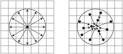
Figure 12.12 A scatter operation takes a pixel’s value and spreads it to the neighboring area, for example by rendering a circular sprite. In a gather, the neighboring values are sampled and used to affect a pixel. The GPU’s pixel shader is optimized to perform gather operations via texture sampling.
Most practical algorithms start with an initial image from one viewpoint. This means that, from the start, some information is missing. The other views of the scene will see parts of surfaces not visible in this single view. As Pesce notes, we should look to do the best we can with what visible samples we have [1390].
Gather techniques have evolved over the years, each improving upon previous work. We present the method by Bukowski et al. [209, 1178] and its solutions to problems encountered. Their scheme generates for each pixel a signed value representing the circle of confusion’s radius, based on the depth. This radius could be derived from camera settings and characteristics, but artists often like to control the effect, so the ranges for the near, focus, and far fields optionally can be specified. The radius’ sign specifies whether the pixel is in the near or far field, with −0.5 < r < 0.5 being in the focus field, where a half-pixel blur is considered in focus.
This buffer containing circle-of-confusion radii is then used to separate the image into two images, near field and the rest, and each is downsampled and blurred in two passes with a separable filter. This separation is performed to address a key problem, that objects in the near field should have blurred edges. If we blurred each pixel based on its radius and output to a single image, the foreground objects could be blurry but with sharp edges. For example, when crossing the silhouette edge from the foreground object to the object in focus, the sample radius will drop to zero, as objects in focus need no blur. This will cause the foreground object’s effect on pixels surrounding it to have an abrupt dropoff, resulting in a sharp edge. See Figure 12.13.

Figure 12.13 Near field blurring. On the left is the original image with no depth-of-field effect. In the middle, pixels in the near field are blurred, but have a sharp edge where adjacent to the focus field. The right shows the effect of using a separate near field image composited atop the more distant content. (Images generated using G3D [209, 1178].)
What we want is to have objects in the near field blur smoothly and produce an effect beyond their borders. This is achieved by writing and blurring the near field pixels in a separate image. In addition, each pixel for this near field image is assigned an alpha value, representing its blend factor, which is also blurred. Joint bilateral filtering and other tests are used when creating the two separate images; see the articles [209, 1178] and code provided there for details. These tests serve several functions, such as, for the far field blur, discarding neighboring objects significantly more distant than the sampled pixel.
After performing the separation and blurring based on the circle of confusion radii, compositing is done. The circle-of-confusion radius is used to linearly interpolate between the original, in-focus image and the far field image. The larger this radius, the more the blurry far field result is used. The alpha coverage value in the near field image is then used to blend the near image over this interpolated result. In this way, the near field’s blurred content properly spreads atop the scene behind. See Figures 12.10 and 12.14.
This algorithm has several simplifications and tweaks to make it look reasonable. Particles may be handled better in other ways, and transparency can cause problems, since these phenomena involve multiple z-depths per pixel. Nonetheless, with the only inputs being a color and depth buffer and using just three post-processing passes, this method is simple and relatively robust. The ideas of sampling based on the circle of confusion and of separating the near and far fields into separate images (or sets of images) is a common theme among a wide range of algorithms that have been developed to simulate depth of field. We will discuss a few newer approaches used in video games (as the preceding method is), since such methods need to be efficient, be robust, and have a predictable cost.

Figure 12.14 Depth of field in The Witcher 3. Near and far field blur convincingly blended with the focus field. (CD PROJEKT ®, The Witcher ® are registered trademarks of CD PROJEKT Capital Group. The Witcher game © CD PROJEKT S.A. Developed by CD PROJEKT S.A. All rights reserved. The Witcher game is based on the prose of Andrzej Sapkowski. All other copyrights and trademarks are the property of their respective owners.)
The first method uses an approach we will revisit in the next section: motion blur. To return to the idea of the circle of confusion, imagine turning every pixel in the image into its corresponding circle of confusion, its intensity inversely proportional to the circle’s area. Rendering this set of circles in sorted order would give us the best result. This brings us back to the idea of a scatter, and so is generally impractical. It is this mental model that is valuable here. Given a pixel, we want to determine all the circles of confusion that overlap the location and blend these together, in sorted order. See Figure 12.15. Using the maximum circle of confusion radius for the scene, for each pixel we could check each neighbor within this radius and find if its circle of confusion included our current location. All these overlapping-neighbor samples that affect the pixel are then sorted and blended [832, 1390].

Figure 12.15 Overlapping circles of confusion. On the left is a scene with five dots, all in focus. Imagine that the red dot is closest to the viewer, in the near field, followed by the orange dot; the green dot is in the field of focus; and the blue and violet dots are in the far field, in that order. The right figure shows the circles of confusion that result from applying depth of field, with a larger circle having less effect per pixel. Green is unchanged, since it is in focus. The center pixel is overlapped by only the red and orange circles, so these are blended together, red over orange, to give the pixel color.
This approach is the ideal, but sorting the fragments found would be excessively expensive on the GPU. Instead, an approach called “scatter as you gather” is used, where we gather by finding which neighbors would scatter to the pixel’s location. The overlapping neighbor with the lowest z-depth (closest distance) is chosen to represent the nearer image. Any other overlapping neighbors fairly close in z-depth to this have their alpha-blended contributions added in, the average is taken, and the color and alpha are stored in a “foreground” layer. This type of blending requires no sorting. All other overlapping neighbors are similarly summed up and averaged, and the result is put in a separate “background” layer. The foreground and background layers do not correspond to the near and far fields, they are whatever happens to be found for each pixel’s region. The foreground image is then composited over the background image, producing a near field blurring effect. While this approach sounds involved, applying a variety of sampling and filtering techniques makes it efficient. See the presentations by Jimenez [832], Sousa [1681], Sterna [1698], and Courr`eges [293, 294] for a few different implementations, and look at the example in Figure 12.16.
One other approach used in a few older video games is based on the idea of computing heat diffusion. The image is considered as a heat distribution that diffuses outward, with each circle of confusion representing the thermal conductivity of that pixel. An area in focus is a perfect insulator, with no diffusion. Kass et al. [864] describe how to treat a one-dimensional heat diffusion system as a tridiagonal matrix, which can be solved in constant time per sample. Storing and solving this type of matrix works nicely on a compute shader, so practitioners have developed several implementations in which the image is decomposed along each axis into these onedimensional systems [612, 615, 1102, 1476]. The problem of visibility for the circles of confusion is still present, and is typically addressed by generating and compositing separate layers based on depths. This technique does not handle discontinuities in the circle of confusion well, if at all, and so is mostly a curiosity today.
A particular depth-of-field effect is caused by bright light sources or reflections in the frame. A light or specular reflection’s circle of confusion can be considerably brighter than objects near it in the frame, even with the dimming effect of it being spread over an area. While rendering every blurred pixel as a sprite is expensive, these bright sources of light are higher contrast and so more clearly reveal the aperture shape.

Figure 12.16 Near and far depth of field with pentagonal bokeh on the bright reflective pole in the foreground. (Image generated using BakingLab demo, courtesy of Matt Pettineo [1408].)
The rest of the pixels are less differentiated, so the shape is less important. Sometimes the term “bokeh” is (incorrectly) used to describe just these bright areas. Detecting areas of high contrast and rendering just these few bright pixels as sprites, while using a gather technique for the rest of the pixels, gives a result with a defined bokeh while also being efficient [1229, 1400, 1517]. See Figure 12.16. Compute shaders can also be brought to bear, creating high-quality summed-area tables for gather depth of field and efficient splatting for bokeh [764].
We have presented but a few of the many approaches to rendering depth-of-field and bright bokeh effects, describing some techniques used to make the process efficient. Stochastic rasterization, light field processing, and other methods have also been explored. The article by Vaidyanathan et al. [1806] summarizes previous work, and McGuire [1178] gives a summary of some implementations.
12.5 Motion Blur
To render convincing sequences of images, it is important to have a frame rate that is steady and high enough. Smooth and continuous motion is preferable, and too low a frame rate is experienced as jerky motion. Films display at 24 FPS, but theaters are dark and the temporal response of the eye is less sensitive to flicker in dim light. Also, movie projectors change the image at 24 FPS but reduce flickering by redisplaying each image 2–4 times before displaying the next. Perhaps most important, each film frame normally is a motion blurred image; by default, interactive graphics images are not.
In a movie, motion blur comes from the movement of an object across the screen during a frame or from camera motion. The effect comes from the time a camera’s shutter is open for 1/40 to 1/60 of a second during the 1/24 of a second spent on that frame. We are used to seeing this blur in films and consider it normal, so we expect to also see it in video games. Having the shutter be open for 1/500 of a second or less can give a hyperkinetic effect, first seen in films such as Gladiator and Saving Private Ryan.

Figure 12.17 On the left, the camera is fixed and the car is blurry. On the right, the camera tracks the car and the background then is blurry. (Images courtesy of Morgan McGuire et al. [1173].)
Rapidly moving objects appear jerky without motion blur, “jumping” by many pixels between frames. This can be thought of as a type of aliasing, similar to jaggies, but temporal rather than spatial in nature. Motion blur can be thought of as antialiasing in the time domain. Just as increasing display resolution can reduce jaggies but not eliminate them, increasing frame rate does not eliminate the need for motion blur. Video games are characterized by rapid motion of the camera and objects, so motion blur can significantly improve their visuals. In fact, 30 FPS with motion blur often looks better than 60 FPS without [51, 437, 584].
Motion blur depends on relative movement. If an object moves from left to right across the screen, it is blurred horizontally on the screen. If the camera is tracking a moving object, the object does not blur—the background does. See Figure 12.17. This is how it works for real-world cameras, and a good director knows to film a shot so that the area of interest is in focus and unblurred.
Similar to depth of field, accumulating a series of images provides a way to create motion blur [637]. A frame has a duration when the shutter is open. The scene is rendered at various times in this span, with the camera and objects repositioned for each. The resulting images are blended together, giving a blurred image where objects are moving relative to the camera’s view. For real-time rendering such a process is normally counterproductive, as it can lower the frame rate considerably. Also, if objects move rapidly, artifacts are visible whenever the individual images become discernible. Figure 12.7 on page 525 also shows this problem. Stochastic rasterization can avoid the ghosting artifacts seen when multiple images are blended, producing noise instead [621, 832].
If what is desired is the suggestion of movement instead of pure realism, the accumulation concept can be used in a clever way. Imagine that eight frames of a model in motion have been generated and summed to a high-precision buffer, which is then averaged and displayed. On the ninth frame, the model is rendered again and accumulated, but also at this time the first frame’s rendering is performed again and subtracted from the summed result. The buffer now has eight frames of a blurred model, frames 2 through 9. On the next frame, we subtract frame 2 and add in frame 10, again giving the sum of eight frames, 3 through 10. This gives a highly blurred artistic effect, at the cost of rendering the scene twice each frame [1192].
Faster techniques than rendering the frame multiple times are needed for real-time graphics. That depth of field and motion blur can both be rendered by averaging a set of views shows the similarity between the two phenomena. To render these efficiently, both effects need to scatter their samples to neighboring pixels, but we will normally gather. They also need to work with multiple layers of varying blurs, and reconstruct occluded areas given a single starting frame’s contents.
There are a few different sources of motion blur, and each has methods that can be applied to it. These can be categorized as camera orientation changes, camera position changes, object position changes, and object orientation changes, in roughly increasing order of complexity. If the camera maintains its position, the entire world can be thought of as a skybox surrounding the viewer (Section 13.3). Changes in just orientation create blurs that have a direction to them, on the image as a whole. Given a direction and a speed, we sample at each pixel along this direction, with the speed determining the filter’s width. Such directional blurring is called line integral convolution (LIC) [219, 703], and it is also used for visualizing fluid flow. Mitchell [1221] discusses motion-blurring cubic environment maps for a given direction of motion. If the camera is rotating along its view axis, a circular blur is used, with the direction and speed at each pixel changing relative to the center of rotation [1821].
If the camera’s position is changing, parallax comes into play, e.g., distant objects move less rapidly and so will blur less. When the camera is moving forward, parallax might be ignored. A radial blur may be sufficient and can be exaggerated for dramatic effect. Figure 12.18 shows an example.
To increase realism, say for a race game, we need a blur that properly computes the motion of each object. If moving sideways while looking forward, called a pan in computer graphics, 1 the depth buffer informs us as to how much each object should be blurred. The closer the object, the more blurred. If moving forward, the amount of motion is more complex. Rosado [1509] describes using the previous frame’s camera view matrices to compute velocity on the fly. The idea is to transform a pixel’s screen location and depth back to a world-space location, then transform this world point using the previous frame’s camera to a screen location. The difference between these screen-space locations is the velocity vector, which is used to blur the image for that pixel. Composited objects can be rendered at quarter-screen size, both to save on pixel processing and to filter out sampling noise [1428].
The situation is more complex if objects are moving independently of one another. One straightforward, but limited, method is to model and render the blur itself. This is the rationale for drawing line segments to represent moving particles. The concept can be extended to other objects. Imagine a sword slicing through the air. Before and behind the blade, two polygons are added along its edge. These could be modeled or generated on the fly. These polygons use an alpha opacity per vertex, so that where a polygon meets the sword, it is fully opaque, and at the outer edge of the polygon, the alpha is fully transparent. The idea is that the model has transparency to it in the direction of movement, simulating the effect that the sword covers these pixels for only part of the time the (imaginary) shutter is open.

Figure 12.18 Radial blurring to enhance the feeling of motion. (Image from “Assassin’s Creed,” courtesy of Ubisoft.)
This method can work for simple models such as a swinging sword blade, but textures, highlights, and other features should also be blurred. Each surface that is moving can be thought of as individual samples. We would like to scatter these samples, and early approaches to motion blur did so, by expanding the geometry in the direction of movement [584, 1681]. Such geometrical manipulation is expensive, so scatter-as-you-gather approaches have been developed. For depth of field we expanded each sample to the radius of its circle of confusion. For moving samples we instead stretch each sample along its path traveled during the frame, similar to LIC. A fastmoving sample covers more area, so has less of an effect at each location. In theory we could take all samples in a scene and draw them as semitransparent line segments, in sorted order. A visualization is shown in Figure 12.19. As more samples are taken, the resulting blur has a smooth transparent gradient on its leading and trailing edges, as with our sword example.

Figure 12.19 On the left, a single sample moving horizontally gives a transparent result. On the right, seven samples give a tapering effect, as fewer samples cover the outer areas. The area in the middle is opaque, as it is always covered by some sample during the whole frame. (After Jimenez [832].)
To use this idea, we need to know the velocity of each pixel’s surface. A tool that has seen wide adoption is use of a velocity buffer [584]. To create this buffer, interpolate the screen-space velocity at each vertex of the model. The velocity can be computed by having two modeling matrices applied to the model, one for the previous frame and one for the current. The vertex shader program computes the difference in positions and transforms this vector to relative screen-space coordinates. A visualization is shown in Figure 12.20. Wronski [1912] discusses deriving velocity buffers and combining motion blur with temporal antialiasing. Courr`eges [294] briefly notes how DOOM (2016) implements this combination, comparing results.
Once the velocity buffer is formed, the speed of each object at each pixel is known. The unblurred image is also rendered. Note that we encounter a similar problem with motion blur as we did with depth of field, that all data needed to compute the effect is not available from a single image. For depth of field the ideal is to have multiple views averaged together, and some of those views will include objects not seen in others. For interactive motion blur we take a single frame out of a timed sequence and use it as the representative image. We use these data as best we can, but it is important to realize that all the data needed are not always there, which can create artifacts.
Given this frame and the velocity buffer, we can reconstruct what objects affect each pixel, using a scatter-as-you-gather system for motion blur. We begin with the approach described by McGuire et al. [208, 1173], and developed further by Sousa [1681] and Jimenez [832] (Pettineo [1408] provides code). In the first pass, the maximum velocity is computed for each section of the screen, e.g., each 8 × 8 pixel tile (Section 23.1). The result is a buffer with a maximum velocity per tile, a vector with direction and magnitude. In the second pass, a 3 × 3 area of this tile-result buffer is examined for each tile, in order to find the highest maximum. This pass ensures that a rapidly moving object in a tile will be accounted for by neighboring tiles. That is, our initial static view of the scene will be turned into an image where the objects are blurred. These blurs can overlap into neighboring tiles, so such tiles must examine an area wide enough to find these moving objects.

Figure 12.20 Motion blur due to object and camera movement. Visualizations of the depth and velocity buffers are inset. (Images courtesy of Morgan McGuire et al. [1173].)
In the final pass the motion blurred image is computed. Similar to depth of field, the neighborhood of each pixel is examined for samples that may be moving rapidly and overlap the pixel. The difference is that each sample has its own velocity, along its own path. Different approaches have been developed to filter and blend the relevant samples. One method uses the magnitude of the largest velocity to determine the direction and width of the kernel. If this velocity is less than half a pixel, no motion blur is needed [1173]. Otherwise, the image is sampled along the direction of maximum velocity. Note that occlusion is important here, as it was with depth of field. A rapidly moving model behind a static object should not have its blur effect bleed over atop this object. If a neighboring sample’s distance is found to be near enough to the pixel’s z-depth, it is considered visible. These samples are blended together to form the foreground’s contribution.
In Figure 12.19 there are three zones for the motion blurred object. The opaque area is fully covered by the foreground object, so needs no further blending. The outer blur areas have, in the original image (the top row of seven blue pixels), a background color available at those pixels over which the foreground can be blended. The inner blur areas, however, do not contain the background, as the original image shows only the foreground. For these pixels, the background is estimated by filtering the neighbor pixels sampled that are not in the foreground, on the grounds that any estimate of the background is better than nothing. An example is shown in Figure 12.20.
There are several sampling and filtering methods that are used to improve the look of this approach. To avoid ghosting, sample locations are randomly jittered half a pixel [1173]. In the outer blur area we have the correct background, but blurring this a bit avoids a jarring discontinuity with the inner blur’s estimated background [832]. An object at a pixel may be moving in a different direction than the dominant velocity for its set of 3×3 tiles, so a different filtering method may be used in such situations [621]. Bukowski et al. [208] provide other implementation details and discuss scaling the approach for different platforms.
This approach works reasonably well for motion blur, but other systems are certainly possible, trading off between quality and performance. For example, Andreev [51] uses a velocity buffer and motion blur in order to interpolate between frames rendered at 30 FPS, effectively giving a 60 FPS frame rate. Another concept is to combine motion blur and depth of field into a single system. The key idea is combining the velocity vector and circle of confusion to obtain a unified blurring kernel [1390, 1391, 1679, 1681].
Other approaches have been examined, and research will continue as the capabilities and performance of GPUs improve. As an example, Munkberg et al. [1247] use stochastic and interleaved sampling to render depth of field and motion blur at low sampling rates. In a subsequent pass, they use a fast reconstruction technique [682] to reduce sampling artifacts and recover the smooth properties of motion blur and depth of field.
In a video game the player’s experience is usually not like watching a film, but rather is under their direct control, with the view changing in an unpredictable way. Under these circumstances motion blur can sometimes be applied poorly if done in a purely camera-based manner. For example, in first-person shooter games, some users find blur from rotation distracting or a source of motion sickness. In Call of Duty: Advanced Warfare onward, there is an option to remove motion blur due to camera rotation, so that the effect is applied only to moving objects. The art team removes rotational blur during gameplay, turning it on for some cinematic sequences. Translational motion blur is still used, as it helps convey speed while running. Alternatively, art direction can be used to modify what is motion blurred, in ways a physical film camera cannot emulate. Say a spaceship moves into the user’s view and the camera does not track it, i.e., the player does not turn their head. Using standard motion blur, the ship will be blurry, even though the player’s eyes are following it. If we assume the player will track an object, we can adjust our algorithm accordingly, blurring the background as the viewer’s eyes follow it and keeping the object unblurred.
Eye tracking devices and higher frame rates may help improve the application of motion blur or eliminate it altogether. However, the effect invokes a cinematic feel, so it may continue to find use in this way or for other reasons, such as connoting illness or dizziness. Motion blur is likely to find continued use, and applying it can be as much art as science.
Further Reading and Resources
Several textbooks are dedicated to traditional image processing, such as Gonzalez and Woods [559]. In particular, we want to note Szeliski’s Computer Vision: Algorithms and Applications [1729], as it discusses image processing and many other topics and how they relate to synthetic rendering. The electronic version of this book is free for download; see our website realtimerendering.com for the link. The course notes by Paris et al. [1355] provide a formal introduction to bilateral filters, also giving numerous examples of their use.
The articles by McGuire et al. [208, 1173] and Guertin et al. [621] are lucid expositions of their respective work on motion blur; code is available for their implementations. Navarro et al. [1263] provide a thorough report on motion blur for both interactive and batch applications. Jimenez [832] gives a detailed, well-illustrated account of filtering and sampling problems and solutions involved in bokeh, motion blur, bloom, and other cinematic effects. Wronski [1918] discusses restructuring a complex post-processing pipeline for efficiency. For more about simulating a range of optical lens effects, see the lectures presented in a SIGGRAPH course organized by Gotanda [575].
1 In cinematography a pan means rotating the camera left or right without changing position. Moving sideways is to “truck,” and vertically to “pedestal.”