
Chapter 7

Using Imperfect FX Elements
FX elements, in the form of stock footage or footage that is shot for a particular project, is a common staple of visual effects compositing. Yet, the elements are rarely perfect and require as much attention as other compositing tasks. If an FX element is unavailable, it’s often possible to replicate the desired phenomena with particle simulation tools or effects. Particle simulations are able to replicate such natural occurrences as falling dust, rising smoke, burning fire, and falling rain. These are precisely the types of elements that are used to make the visual effects shots more exciting.
This chapter includes the following critical information:
• FX elements overview
• Methods for keying out unwanted FX backgrounds
• Merging FX elements with new backgrounds
• Generating particle simulations
• Adjusting particles to emulate an FX element
FX Elements Overview
As discussed, stock footage is pre-shot motion picture of video footage available via a library that may be licensed for use on a project. Visual effects compositing often makes use of stock footage. In fact, a subset of stock footage, known as VFX or FX elements, is designed specifically for such compositing. The FX elements often contain naturally occurring phenomenon that is difficult or time-consuming to realistically replicate in the composite or in an external 3D program. For example, the FX elements may feature falling dust, dirt, or debris, fire in various forms, isolated explosions, lens flares, rain or water splashes, or different types of smoke.
A quality FX element possesses a high resolution and places the specific effect against a black or other solid-colored background, making the separation of the effect efficient. Large studios or well-budgeted productions may shoot their own FX elements in order to exert the maximum amount of control. When working with FX elements from a library, it’s often necessary to make adjustments to the footage to make the composite successful. Ultimately, an FX element is rarely perfect for an intended use. By the same token, you can make adjustments to an FX element using common compositing effects or tools to make a substandard element function in a quality manner.
When an FX element is not available, it is possible to generate basic phenomena in the compositing program with particle systems. A particle system simulates the motion of myriad particles reacting to natural forces such as gravity in wind. Particle systems are able to replicate fire, explosions, rain, dust, and sparks. Although the particle systems built into compositing programs are not as advanced as counterparts in dedicated 3D programs, you can still create serviceable simulations for commonly needed elements.
FX Element Problems and Solutions
Table 7.1 lists common problems and solutions for working with FX elements.
Table 7.1
| Problem | Solution |
| Low-resolution FX element | Low resolution is not always a detriment for some elements, such as fog, smoke, or rain. You can scale up the footage. If pixelation is visible, apply an additional blur. Because a fog, smoke, or rain element necessitates a low opacity, the additional blur is perfectly suitable. |
| “Dirty” background | If an FX element lacks a “clean” background that cannot be easily removed, apply the various keying tricks discussed in Chapter 1. For example, try different keyers, mask, rotoscope, create custom luma keys, and so on. Note that many elements only require the proper blending mode selection and don’t require that the background be converted to transparent alpha. For example, smoke shot against a dark background only requires the Screen blending mode. |
| Improper camera angle | It’s not unusual for an FX element to be shot at an angle that doesn’t match the shot in which you wish to place it. In this situation, convert the footage to a card and position, rotate, and scale the card in the compositing program’s 3D environment. Cards are demonstrated in Chapter 6. |
| Improper duration | An FX element may be too short for a composite. You can combine multiple iterations of the elements and blend them together by animating opacity. In addition, you can randomize the iterations by adjusting each iteration’s scale, rotation, or position. Compositing programs allow you to mirror the X or Y scale by entering a negative value, such as −100. |
| Improper speed | An FX element may be moving too fast or too slow. Apply time warping effects or tools to change the speed. You can also use time warping to adjust the element duration. Use caution, as time warping can lead to visible artifacts, such as judder. |
Stock FX Element Challenge
Figure 7.1 shows several frames from the Smoke.##.png image sequence. Although the original video was not designed as an FX element, we can use it as example of footage that can be made into a useful element despite its limitations. We will add this smoke to the Chimneys.##.png footage, which is illustrated by Figure 7.2. Table 7.2 also describes the strengths and weaknesses of the smoke image sequence.

Figure 7.1 Two frames from a video featuring smoke pouring out of a chimney. Image sequence adapted from “Smoke” by Oleksii Leonov and is licensed under Creative Commons Attribution 2.0 Generic (CC BY 2.0).

Figure 7.2 An image sequence featuring a series of house chimneys will receive the smoke element. Image sequence adapted from “Chimneys” photo by Dominic Mitchell and is licensed under Creative Commons Attribution 2.0 Generic (CC BY 2.0).
Table 7.2
| Strengths | Strengths |
| There is good color contrast between the smoke and the blue sky. As such, you can use a chroma keyer to remove the sky. | The background includes dark tree limbs at the bottom of frame and a bright diagonal cloud in the sky, both of which will interfere with chroma keying. |
| The sequence is 150 frames long, giving flexibility when adding the smoke to a new background that has a shorter duration. | The smoke runs in reverse and moves quickly, requiring time warping. |
| Because the smoke will be added to a number of chimneys far from the camera, a large element resolution is not required. Because the element features smoke, we can add additional blur and reduce the smoke opacity to disguise any limitations. | The resolution is small at 500×282, giving us relatively few pixels to work with. |
Layer-Based Solution for FX Element Challenge
You can use a keyer to remove the background of the smoke image sequence. However, instead of using the Keylight effect as we did in Chapter 1, we can use a more specialized keyer that is more suited for soft-edged foregrounds. Follow these steps:
1. Create a new project. Import the Project-FilesPlatesSmokeSmoke.##.png image sequence. Interpret the footage frame rate as 24 fps. Create a new composition that matches the image sequence. Set the composition’s resolution to 500×282, duration to 150, and frame rate to 24. Place the image sequence in the new composition.
2. With the smoke layer selected, choose Effect > Keying > Color Difference Key. The Color Difference Key keyer works by combining to partial alpha mattes to create a single output matte. The keyer generally produces good results when working with a soft foreground, such as smoke. Temporarily turn off the Color Difference Key in the Effect Controls panel. Select the effect’s Key Color eyedropper and sample a blue portion of the sky in the Composition view. Turn the Color Difference Key back on.
3. The Color Difference Key carries an alpha matte preview at the top-right of its properties list. By default, the final alpha matte is displayed. However, you can show the A and B partial mattes by clicking the A and B buttons. To return to the output matte, click the a button. Initially, the output matte is low-contrast. To improve the matte, click the middle eyedropper button and LMB-click on the matte preview in the Composition view to clean the gray noise in the background. For example, LMB-click in the portion of the sky that carries gray pixels. You can LMB-click multiple times with each click updating the alpha matte. The matte preview updates, as well as the background opacity in the composition view. The middle eyedropper remotely drives the effect’s Matte In Black property. Any alpha value less then the Matte In Black property value is pushed down to 0-black (100% transparency).
4. Click the bottom eyedropper button and LMB-click on the matte preview in the Composition view to clean the gray noise in the foreground smoke. The eyedropper remotely drives the Matte In White property. It’s okay to leave some semi-transparency in the smoke (Figure 7.3). (The Matte In Black and Matte In White properties are similar to the Clip Black and Clip White properties carried by the Keylight effect, discussed in Chapter 1.)

Figure 7.3 Top: The Color Difference Key preview swatches, with the output alpha matte shown on the right. The Matte In Black and Matte In White In values are adjusted via eyedroppers to increase the matte contrast. Bottom: Result of the keyer.
5. Play back the timeline. The footage runs backwards. You can reverse the footage by selecting the layer and pressing Ctrl/Cmd+Alt/Opt+R. A reversed layer is given red hash marks along the footage bar. You can further adjust the alpha matte created by the Color Difference Key by adjusting the In Black, In White, Gamma, Out Black, and Out White properties of the partial A and partial B mattes. Each adjustment will alter the matte, so feedback is immediate. That said, after setting the Matte In Black and Matte In White values, the alpha matte is ready to use. To see the matte more clearly, switch the Composition view’s Show Channel menu to Alpha (Figure 7.4).

Figure 7.4 The alpha channel after the adjustment of Matte In Black and Matte In White. Note that the center of the smoke is opaque and the smoke edges are semi-opaque.
6. At this juncture, the trees, chimney, and diagonal cloud remain in the background. They require rotoscoping to remove. Return the Show Channel menu to RGB. With the layer selected, use the Pen tool to draw a closed mask that surrounds the trees, the chimney, and the remaining clouds at the bottom of frame (Figure 7.5). Make the mask subtractive by changing the mask blending mode menu to Subtract. The menu is to the right of the mask name in the layer outline. Increase the Mask Feather.

Figure 7.5 Two subtractive masks are drawn to remove the unwanted trees, chimney, and remaining background clouds
7. Go to frame 0. Using the Pen tool, draw a second closed mask that surrounds the diagonal cloud at the left side of the frame (see Figure 7.5 on the previous page). Set the mask blending mode to Subtract and increase the Mask Feather value. This mask requires animation due to the fluctuation of the foreground smoke. Activate the Time icon beside the Mask Path property for the mask. Go to later frames and adjust the mask shape. A keyframe every 5 to 10 frames is necessary to keep the mask from cutting heavily into the foreground smoke.
8. Rename the composition Smoke. Create a new composition that has a resolution of1920x1440, a frame rate of 24 fps, and a duration of 72 frames. Name the new composition Chimneys. Import the Project-FilesPlatesChimneysChimneys.##.png image sequence. Interpret the footage frame rate as 24 fps. LMB-drag the new sequence from the Project panel into the Chimneys composition. The sequence features a high-angle, static shot of a rooftops with chimneys.
9. LMB-drag the Smoke composition from the Project panel to the Chimneys composition, placing it on top of the layer outline. Interactively move the nested smoke so that it lines up with a chimney that carries the cylindrical pipes. Alter the scale of the nested smoke so it fits the chimney. Because the Smoke composition is significantly longer in duration than the Chimney’s composition, you can LMB-drag the smoke layer’s footage bar left or right to choose a different section of smoke.
10. The smoke retains a dark core (left side of Figure 7.6). This does not integrate with the new background. Add a Curves effect to the smoke layer (Effect > Color Correction > Curves). Adjust the effect’s curve so that the brightness and darkness of the smoke is inverted (right side of Figure 7.6). You can do this by pulling the curve’s left point higher than the curve’s right point (Figure 7.7).

Figure 7.6 Left: the smoke is placed over a chimney but retains a dark core. Right: the smoke is inverted with a Curves effect.

Figure 7.7 A Curves effect is adjusted to invert the smoke, making the core appear brighter than the edges.
11. Play back. When the smoke leaves the edge of the nested layer frame, it is suddenly cut off. To avoid this, use the Pen tool to draw an irregular mask near the edges of the layer (Figure 7.8). Increase the Mask Feather so that the smoke fades as it approaches the layer edges. Play back and adjust the mask shape and the Mask Feather until the result is satisfactory.

Figure 7.8 An irregular mask is drawn around the smoke layer. A large Mask Feather allows the smoke to fade out near the edges. The chimney image sequence is temporarily hidden. Note the short motion path in the center, indicating that the layer is animated moving left and right to stay centered over a particular chimney.
12. The bottom of the smoke column may appear to drift left or right and may not appear rooted to the chimney. Optionally, you can animate the smoke layer’s Position values to keep the smoke column centered. Only a few keyframes with minor change in the Position X value are necessary.
13. Lower the smoke layer’s Opacity to make the smoke more subtle. Change the smoke layer’s Blending Mode menu to Lighten. This discards any remaining dark edge of the smoke so that the result is more consistently white, as if the smoke is mostly water vapor. Play back. The smoke should be somewhat difficult to see when stopped on a frame but easy to see when the composition is played back.
14. To further improve the smoke integration, you can go back to the Smoke composition and fine-tune all the property values of the Color Difference Key effect. Make additional adjustments to the Matte In Black and Matte In White properties. You can also adjust any of the Partial A or Partial B properties. For example, the final version of the project included with the tutorial files uses the following, non-default settings:
Partial A In White = 254
Partial A Out White = 217
Partial B In White = 251
Matte In Black = 119
Matte In White = 236
15. Return to the Chimneys composition. Repeat the process outlined in steps 10 through 14 to add several more iterations of smoke to several other chimneys. LMB-drag the footage bar of each new smoke layer so that it uses a unique portion of the smoke.
16. At this stage, the smoke columns may occlude the cylindrical ends of the chimneys. This may make the perspective of the smoke columns appear incorrect. To solve this, you can create a paint fix patch and place it on top of the composition. Select the chimney sequence layer and duplicate it. Move the duplicated layer to the top of the layer outline. With the new layer selected, use the Pen tool to draw several, closed masks that separate the tops of the chimneys where smoke is placed. By creating these patches and placing them on top, they cover up any smoke that is in the incorrect location (Figure 7.9).

Figure 7.9 Two additional iterations of smoke are added. They are placed under an additional copy of the chimney sequence that is masked to create paint fix patches of the chimney tops. The lowest chimney layer is temporarily hidden.
17. As a final step, we can add smoke to the left foreground of the frame. Add one more iteration of the smoke to the composition and make it the highest layer. Set the layer’s Scale to 700%. Set the Blending Mode menu to Lighten. Reduce the Opacity to 25%. Add an irregular mask to the layer with a large Mask Feather to further soften the smoke as it reaches the frame edge. Position and rotate the layer so that the smoke rises up through the frame on the left side. Because the smoke layer possesses a small resolution, pixelation becomes visible. To disguise this, add a Fast Blur effect to the layer (Effect > Blur & Sharpen > Fast Blur) and set the Blurriness to 10. The extra blur also makes it appear as if the foreground smoke is out-of-focus due to a slightly narrow depth-of-field. Play back. The composition is complete (Figure 7.10).

Figure 7.10 Top: Final placement of four smoke layers with the one on the left scaled up by 700%. Bottom: Final composite. The smoke is easily seen when the timeline is played back.
A chart detailing the layer workflow is illustrated by Figure 7.11. The project is included with the tutorial files as Project-FilesaeFilesChapter5FXElementChallengeFinal.aep.

Figure 7.11 Compositions, layers, and effects used in After Effects. Compositions are shown as blue boxes. Layers are numbered and written in bold type. Effects are listed beside each layer. The arrow indicates nesting.
Node-Based Solution for FX Element Challenge
You can use a keyer to remove the background of the smoke image sequence. However, instead of using the Primatte tool as we did in Chapter 1, we can use a simple keyer that is nevertheless able to remove the background with fewer adjustments.
Keying and Merging the Smoke
When applying a keyer, premultiplication issues can affect the way in which you construct the network. Follow these steps:
1. Create a new project and a new Loader. Import the Project-FilesPlatesSmokeSmoke.##.png image sequence. The footage is running backwards. To reverse it, select the Reverse checkbox carried by the Loader. Choose File > Preferences and set the project frame rate to 24 fps. Set the Global End Time to 149.
2. Choose Tools > Matte > Chroma Keyer. Connect the output of the Loader to the input of the Chroma Keyer tool. Connect the Chroma Keyer to a Display view. In contrast to the Primatte tool, the Chroma Keyer has few options. As a keyer, it operates in two modes, as set by the buttons at the top of the Tools > Chroma Key tab: Chroma and Color. The Chroma mode creates an alpha matte based on RGB values set by the tool’s range sliders. The Color mode creates a matte based on the hue values of the range sliders (as such, hue is separated from saturation and value). With the tool set to Chroma, lower the Red High value. You can do this by LMB-dragging the right side of the Red Low/Red High slider. The alpha matte updates so that the sky is removed and the smoke is saved. This is due to a high red content in the smoke and a low red content in the sky. The Chroma Keyer works in an opposite fashion than many keyers, whereby the matte is inverted. For example, if you return Red High to 1.0 and lower the Blue High value, the blue of the sky is saved and the smoke is discarded.
3. Return the Blue High property to 1.0 and set the Red High property to 0.44. This removes the majority of the background. You can examine the alpha channel by pressing the A key while the Display view is selected. While adjusting the Chroma Keyer tool, you want to make sure that the smoke core does not develop holes. For example, a slightly higher Red High value causes this to happen. To best judge the results, play back the time ruler while looking at the alpha channel and the RGB channels. In general, the Chroma Keyer tool tends to leave the foreground with a hard, pixelated edge. You can soften this by switching to the tool’s Tools > Matte tab and raising the Matte Blur parameter value. For example, Figure 7.12 uses a Matte Blur value of 10.

Figure 7.12 Top: Result of the Chroma Keyer tool. Bottom: Same frame, as seen in the alpha channel.
4. The Chroma Keyers tool is unable to remove the trees at the bottom of the frame, as well as the chimney and a diagonal cloud on the frame-left side. Hence, it is necessary to rotoscope these unwanted elements. Create two Polygon tools (Tools > Mask > Polygon). Connect the output of the first Polygon tool to the Garbage Matte input of the Chroma Keyer tool. With the connected Polygon tool selected, draw a closed mask that surrounds the trees and chimneys at the bottom of the frame (Figure 7.13). Those elements are cut out. Connect the output of the second Polygon tool to the Effect Mask input of the first Polygon tool. Use Figure 7.18 as reference for the final tool network. With the second Polygon tool selected, draw a closed mask that removes the diagonal cloud at the left side of the frame (Figure 7.13). The second mask requires animation so that it doesn’t cut into the smoke. A keyframe every five to ten frames is sufficient for the mask to follow the edge of the smoke.

Figure 7.13 Two masks are drawn with two Polygon tools. When connected to the Garbage Matte input of the Chroma Keyer, the masks become subtractive.
5. Raise the Soft Edge value for each Polygon tool so that the masks softly erode into the edge of the smoke. At this stage, the smoke has a dark central core and a bright edge. In order to integrate the smoke into a new background, we’ll need to brighten the core. Choose Tools > Color > Color Curves and Tools > Matte > Alpha Multiply. Connect the output of the Chroma Keyer tool to the input of the Color Curves tool. Connect the output of the Color Curves tool to the Alpha Multiply tool. Connect the Color Curves tool to a Display view. Deselect the Color Curves tool’s Alpha checkbox. Invert the Color Curves tool’s curve by moving the left point up and the right point down (Figure 7.14). This brightens the smoke core and darkens the smoke edges. At the same time, the empty area of the frame becomes white. To prevent this, we can premultiply the alpha values by the RGB values. This is carried out by the Alpha Multiply tool. Connect the Alpha Multiply tool to a Display view. The unwanted white goes away (Figure 7.15).

Figure 7.14 The curves of a Color Curves tool is inverted, thus brightening the smoke core.

Figure 7.15 Result of the Color Curves and Alpha Multiply tools.
6. Create a new Loader and import the Project-FilesPlatesChimneysChimneys.##.png image sequence. The sequence features a high-angle, static shot of rooftops with chimneys. Change the Global End Time to 71. (The new sequence is only 72 frames long.) Create a new Merge tool. Connect the output of the Alpha Multiply tool to the Foreground of the Merge tool. Connect the output of the new Loader to the Background of the Merge tool. Connect the Merge tool to a Display view. The smoke, which is at a smaller resolution, appears on the center of the chimney footage. The area outside the smoke’s bounding box appears semi-transparent white due to problems with the premultiplication workflow (Figure 7.16). To remove the extra white, draw a closed mask within the smoke’s bounding box. After the mask is drawn, connect the associated mask tool to the Merge tool’s Effect Mask input. For example, in Figure 7.17, a BSpline tool is used to draw an irregular mask. Increase the mask tool’s Soft Edge value to fade the smoke out as it reaches the mask edge. To prevent a white line from appearing outside the mask, reduce the mask tool’s Border Width, which erodes the mask inwards.

Figure 7.16 The smoke is merged with the new background, with the smoke appearing smaller and in the center. The extra white along the edges is due to a premultiplication error.

Figure 7.17 Close-up of BSpline mask drawn to remove the extraneous white surrounding the smoke.
7. Select the Merge tool and reduce the Blend value to fade out the smoke. The smoke should be barely visible when looking at a single frame but easily seen when playing back the time ruler. Change the Merge tool’s Apply Mode menu to Lighten. This removes the darker edges on the smoke.
8. The smoke is positioned in the center of frame and does not line up to any chimney in the background. You can move the smoke by using the transform handle provided by the Merge tool. However, if you try this, the mask will not travel with the smoke. To avoid this you can connect the Merge transform with the Mask transform. Go to frame 0. With the Merge tool selected, RMB-click over the Center property name and choose Animate. A single keyframe is laid down. Select the newest mask tool. RMB-click over the mask tool’s Center parameter name and choose Connect To > Path1 > Position. This creates an expression, where the Center parameter of the mask automatically derives its values from the Center parameter of the Merge tool. Select the Merge tool. Interactively move the smoke. The mask follows. Position the smoke over a chimney at the right side of frame. Select a chimney that carries the cylindrical clay pipes. You can adjust the Merge tool’s Size value if the smoke appears too large or too small in comparison to the selected chimney.
9. Because the smoke footage is far longer in duration than the chimney sequence, you can choose different portions of smoke to appear on the time ruler. To do this, select the Loader that imports the smoke and adjust the Trim Out value. For example, while on frame 0, lower the Trim Out value from 149 to 74. This causes the smoke sequence to start 75 frames later. After you’ve adjusted the Trim Value, the composition is complete. Figure 7.18 illustrates the smoke’s final integration.

Figure 7.18 Top: Frame 0, showing final smoke integration. Bottom: Frame 40.
The final tool network is illustrated by Figure 7.19. A chart detailing the layer workflow is illustrated by Figure 7.20. The project is included with the tutorial files as Project-FilescompFilesChapter7FXElementChallengeFinal.aep.
Figure 7.19 The final tool network.

Figure 7.20 Simplified representation of the Fusion node network. Colored boxes represent branches of the network. Specific tools are listed under each branch with low-numbered tools existing farther upstream. Purple arrows indicate the connections of masks.
Rendering and Combining Smoke Iterations
There are several ways to add multiple iterations of the smoke to the Fusion composition. Perhaps the easiest method is to render out the smoke, re-import the render, and re-merge it with the background. You can follow these steps:
1. Using the tool network set up in the previous section, select the AlphaMultiply1 tool. Choose Tools > I/O > Saver. The Save File window opens. Enter SmokeKeyed.00.png into the name field. Navigate to a new directory where you wish to render the new image sequence. Click Save to close the window. The Saver tool is inserted between the AlphaMultiply1 tool and the Merge1 tool. This does not affect the functionality of the prior tool network.
2. Select the Loader1 tool, which imports the smoke sequence. Return the Trim Out property to 149. Change the Global End Time and Render End Time fields, in the TimeView, to 149. Click the nearby Render button. The Render Settings window opens. By default the settings are high-quality. Click the Start Render button. The output of the AlphaMultiply1 tool, with it alpha matte, is rendered.
3. When the render is completed, change the Global End Time and Render End Time back to 71. Create a new Loader and import the recent render. A sample render is included as Project-FilesPlatesSmokeKeyedSmokeKeyed.##.png. Connect the new Loader to a Display view. The alpha transparency is read correctly. However, the smoke crosses the edge of frame and there is a soft white line around the edges. We can mask this out. Create a new BSpline tool. With the new tool selected, draw a closed, irregular mask that cuts off the unwanted edges. Connect the output of the BSpline tool to the Effect Mask input of the new Loader. Adjust the BSpline tool’s Soft Edge and Border Width properties so that the smoke softly fades as it reaches the mask.
4. To add a second iteration of the smoke with an offset time, copy and paste the new BSpline and Loader tools. Open the copied Loader and change the Trim In value to offset the second iteration of the smoke. For example, set the Trim in to 75 so that the second iteration starts at frame 75 instead of 0.
5. Create two Transform tools. Connect the output of one Loader to the input of one Transform tool and the output of the second Loader to the input of the second Transform tool. Use Figure 7.21 as reference for the new tool network. Create a new Merge tool. Connect the outputs of the Transform tool to the Foreground and Background of the Merge tool. The order does not matter. Create a new Merge tool. Connect the output of the prior Merge tool to the Foreground of the new Merge tool. Connect the output of Loader2, which imports the Chimney sequence, to the Background of the newest Merge. Connect the newest Merge tool to a Display view. The smoke is placed over the background.
6. At this point, the two smoke iterations are on top of each other. Go to each Transform tool and change the Center and Scale properties to place each smoke iteration in a unique location. Select the newest Merge tool and change its Apply Mode to Lighten. Adjust the Blend property to fine tune the smoke opacity. Play back. The new composite is complete.
If you wish to add additional iterations of the smoke, you will have to add new branches to the network that includes a Loader with a unique Trim In, a BSpline tool to remove the edges, a Transform tool to position and scale the new smoke, and a Merge tool to combine the smoke with other smoke iterations. Keep in mind that Merge tool can only combine two inputs. However, you can chain together as many Merge tools as necessary. Figure 7.21 illustrates the new network. Figure 7.22 shows two iterations of smoke combined over the background. The project is included with the tutorial files as Project-FilescompFilesChapter7FXElementChallengePart2.aep

Figure 7.21 The new tool network, designed to combine multiple iterations of the smoke. The connection line that extends out of the frame on the left is connected to the Loader that imports the chimneys sequence.
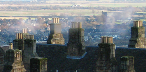
Figure 7.22 Result of the new network, with smoke appearing over two separated chimneys.
Particle FX Challenge
It’s not always practical to use FX elements, either due to budget or time constraints. Hence, compositing programs supply particle simulation tools to replicate common natural phenomena. Such phenomena includes fire, explosions, sparks, rain, falling debris, dust, and smoke. As a challenge, we’ll add steam to the pot of boiling water illustrated by Figure 7.23.

Figure 7.23 An image sequence featuring a boiling pot. Image sequence adapted from “how to boil water” by Matt MacGillivray and is licensed under Creative Commons Attribution 2.0 Generic (CC BY 2.0).
Layer-Based Solution for Particle FX Challenge
After Effects includes several particle simulation effects. Although each effect carries a different set of properties, they all follow the same basic simulation steps: create and position a particle emitter, determine the particle birth rate, size, and rendering style, and adjust forces that affect the way in which the particles move. Note that a particle simulation is rarely used as-is and generally requires the application of additional effects to replicate a particular phenomena. You can follow these steps to create your own simulation:
1. Create a new project. Import the Project-FilesPlatesPotPot.##.png image sequence. Interpret the footage frame rate as 24 fps. Create a new composition that matches the image sequence. Set the composition’s resolution to 1280×720, duration to 48, and frame rate to 24. Set the composition Start Frame to 0001. Place the image sequence in the new composition.
2. Choose New > Layer > Solid and set the solid’s resolution to 1280×720. The solid color does not matter as we will place the simulation on the solid layer. Click OK to close the Solid Settings window. The solid is placed on top of the layer outline. With the solid layer, choose Effect > Simulation > CC Particle World. The effect adds a particle emitter (called a producer) to the Composition view; this is drawn as a red sphere. Interactively LMB-drag the emitter sphere to the center of the pot. Note that the solid color disappears when the effect is applied. The emitter sphere and accompanying grid are drawn for reference and will not appear in final renders.
3. Note that the effect adds an axis cube at the top-left of the view. LMB-drag the cube edges to manipulate the virtual camera that sees the particles. Adjust the axis cube so that the top reads –Y. Continue to adjust the cube and position the emitter so that the green line, which represents the Y axis, points downwards. Continue to adjust the cube so that the grid lines up with the top of the stove (figure 7.24). The grid represents the XZ plane. Note that the CC Particle World effect must be selected for the cube, grid, and emitter to be seen.

Figure 7.24 The axis cube and emitter sphere are adjusted so that the virtual camera emulates the real-world camera. The virtual camera looks down the Y axis at the XZ plane.
4. Play back. Particles are born at the emitter and fall in the –Y direction. This is due to a built-in gravity. Expand the CC Particle World effect’s Physics section (Figure 7.25). Set the Gravity property to –0.5. Play back from frames 1.The particles flow upwards toward the camera in the +Y direction.

Figure 7.25 Physics and Particle section of CC Particle World effect with adjusted properties.
5. At this point, the particles are narrow, yellow lines. Expand the effect’s Particle section. Change the Particle Type menu to Faded Sphere. Set Birth Size to 2. Set Death Size to 5. This causes the sphere particles to grow in size during their lifetime, which is set to 2 seconds via the Longevity property. Reduce the Max Opacity property to 10% to fade the particles out. Change the Birth Color to white and Death Color to black. Play back from frame 1. This creates a sooty smoke-like appearance. To make the simulation more steam-like, set the solid layer’s Blending Mode menu to Screen. The Screen mode ignores the dark areas of the particles (Figure 7.26).

Figure 7.26 Left: Particles rendered with the Fade Sphere type with the image sequence hidden. Right: Particles added to the sequence with the Screen mode. The particle motion is easily seen when the timeline is played back.
6. In the Physics section, set the Animation menu to different options and play back. The Animation menu sets the internal forces used to alter the particle paths outside the separate gravity function. For example, set the menu to Viscous, which allows the particles to rise in a sluggish, semi-random fashion. You can further adjust the simulation with the Velocity and Resistance properties. For example, you can slow the particle by reducing the Velocity below 1.0. You can hide the axis cube, grid, and emitter by deselecting the Position, Radius, Grid, Horizon, and Axis Box properties in the Grid & Guides section.
7. The first particles are born at frame 1 and therefore do not appear in a thick cloud until a later frame. To have the particle simulation start at a negative frame number, LMB-drag the entire footage bar for the solid layer so that its start is pushed before frame 1. LMB-drag the end of the footage bar so that it fills up the remainder of the timeline. Play back. The particle cloud is thick and well-formed on frame 1 of the timeline. To soften the particle cloud, you can add a blur effect. For example, add a Fast Blur effect to the solid layer and set the Blurriness to 50 and select the Repeat Edge Pixels checkbox. The composition is complete. Figure 7.27 shows three frames from the simulation with the image sequence hidden.
If you wish to form the steam into a thicker cloud, you can raise the Birth Rate property above 2. You can also increase the Opacity and change the Birth Color to gray or white. You are also free to color grade the particles by adding color effects to the solid layer. A chart detailing the layer workflow is illustrated by Figure 7.28. The project is included with the tutorial files as Project-FilesaeFilesChapter7ParticleChallengeFinal.aep.

Figure 7.27 Top to bottom: Frames 1, 24, and 48 of final particle simulation with the background hidden.

Figure 7.28 Composition, layers, and effects used in After Effects. Composition is shown as a blue box. Layers are numbered and written in bold type.
Node-Based Solution for Particle FX Challenge
You can follow these steps to create a particle simulation in Fusion:
1. Create a new project. Add the following tools: pEmitter, pDirectionalForce, pTurbulence, and pRender. The tools with a p prefix are particle simulation tools and are located in the Tools > Particles menu. Add the following tools: Camera 3D, Merge 3D, and Renderer 3D. These tools are located in the Tools > 3D menu. We’ll use this set of tools to generate particles, affect their motion, and render them.
2. Connect the output of the pEmitter tool to the pRender tool. Connect the output of the pRender tool to the Merge 3D tool. Connect the Camera 3D tool to the Camera input of the pRender tool. Connect the output of the Merge 3D tool to the Renderer 3D tool. Use Figure 7.34 as reference for the final tool network. Connect the Merge 3D tool to a Display view. The view shows the 3D environment through the lens of the default perspective camera. The camera created by the Camera 3D tool is visible as a camera icon and is located at 0, 0, 0. Set the Global Start Time to 1 and Global End Time to 48. Play back. Particles are born at the emitter location of 0, 0, 0. The particles are drawn as points within the spherical emitter and do not move away from the emitter (Figure 7.29).

Figure 7.29 The Camera 3D camera and pEmitter sphere are placed at 0, 0, 0 by default. The particles are drawn as points and do not move.
3. Select the Camera 3D tool. Using the Move and Rotate buttons added to the Display view, move and rotate the camera away from the emitter so that it points downwards. Select the pEmitter tool. Switch to the tool’s Tools > Style tab. Change the Style menu to NGon. This changes the particles to primitive polygons. In the NGon section, near the bottom of the tab, click the Soft Circular button to make the particles sphere-like. In the Size Controls section, change the Size property to 1.0. Play back. The particles are now larger but still do not move (Figure 7.30).

Figure 7.30 The Camera 3D cameras moved and rotated to point down at the particles, which are changed to NGon spheres.
4. Select the pEmitter tool and return to the Tools > Controls tab. Reduce the Number property to 2. This reduces the number of particles born per frame. Update the tool network so that the pEmitter tool connects to the pDirectionalForce tool, the pDirectionalForce tool connects to the pTurbulence tool, and the pTurbulence tool connects to the pRender tool. Use Figure 7.34 as reference for the final tool network. Tools that carry the force suffix create forces that emulate physical forces in the real work and affect the motion of particles. You must connect the force tools between the pEmitter and pRender tools. Select the pDirectionalForce tool. Change the Direction to 90 and the Strength to 0.02. Play back from the first frame. The particles flow upwards as if buoyant or pushed by wind. (If you want to create a gravity like force, set Direction to −90.) Select the pTurbulence tool, which is also a force tool. Increase the X, Y, and Z Strength to 2. This adds a random motion to the particles when you play back and prevents the particles from flowing in a straight column.
5. Select the connected Display view, RMB-click in the view, and choose Camera > Camera3D1. Select the pRender or Merge 3D tool to see the rendered particles. You can adjust the Camera 3D camera’s view by selecting the Camera 3D tool and using the camera shortcuts in the Display view. You can dolly left/right or up/down by MMB+dragging. You can dolly forward or backward by LMB+MMB-dragging left or right. You can rotate the camera by Alt/Opt+MMB-dragging. Position the Camera 3D camera so that the particles take up a large portion of the top-center frame when played back (Figure 7.31).

Figure 7.31 Particles seen on a late frame through the Camera 3D camera while the Merge 3D tool is selected.
6. To see the final render quality of the particles, connect the Renderer 3D to a Display view. The Renderer 3D tool shows the correct frame and final particle surface quality. Select the pEmitter tool. Return to the Tools > Style tab. Expand the Color Controls section. Locate the horizontal color bar in the Color Over Life Controls subsection. LMB-click the bar at the far-right side. A new triangular handle is inserted. While the new handle is selected, change the color swatch, which is directly below, to black. This causes the particles to slowly change from white to black over their lifespan (which, by default is set to 100 frames via the Lifespan property in the Tools > Controls tab). This will help give the particles variation in their mass when it comes time to combine them with the background (Figure 7.32).

Figure 7.32 Particles rendered with Renderer 3D tool, as seen on frame 24. The color variation is created with the Color Over Life Controls color bar. With this example, the Global In value is set to −25 in order to create a pre-roll.
7. The first particles are born at frame 1. This means that a cloud-like mass will not form until a later frame. To prevent this, you can create a “pre-roll” where particles begin to form at a negative frame number. To do this, select the pRender tool and change the Global In property to a negative value. For example, change the Global In value to −25 so that the particles start to appear twenty-five frames before the first frame is rendered by the time ruler. Play back. The particle mass appears thick on the first frame.
8. Create a Blur tool and a Merge tool. Connect the output of the Renderer 3D tool to the input of the Blur tool. Connect the output of the Blur tool to the Foreground of the Merge tool. Use Figure 7.34 as reference for the final tool network. Create a new Loader and import the Project-FilesPlatesPotPot.##.png image sequence. Connect the output of the Loader to the Background of the Merge tool. Connect the Merge tool to a Display view. The particle steam is added over the new background. By default, the Renderer 3D tool renders the project resolution as set by the Preference window. This is 1920×1080 by default. Hence, the particle render overhangs the background. This gives you the chance to move and scale the particle render to better position it over the pot. To do so, select the Merge 3D tool and use the transform handle to move. To scale, change the Merge tool’s Size property.
9. Select the Blur tool and set the Blur Size to 25. This soften the particle render. Select the Merge tool and change the Apply Mode menu to Screen. This discards the darkest areas of the particle render. To make the particle steam less visible, reduce the Merge tool’s Blend value. The steam should be difficult to see on a single frame but should be easy to detect when playing back. The composite is complete. Figure 7.33 shows the pot sequence with and without the particles.

Figure 7.33 Top: Pot sequence without particle steam. Bottom: Sequence with particle steam added. With this example, the Blend value of the Merge tool is set to 0.5. To make the steam more subtle, lower the Blend value.
Figure 7.34 illustrates the final tool network. Figure 7.35 illustrates the tool workflow. The project is included with the tutorial files as Project-FilescompFilesChapter7ParticleChallengeFinal.aep.

Figure 7.34 The final tool network.

Figure 7.35 Simplified representation of the Fusion node network. Colored boxes represent branches of the network. Specific tools are listed under each branch with low-numbered tools existing farther upstream.
Final FX Element Thoughts
Although the perfect FX element may be available as stock footage, more often than not a compositor is forced to adapt an imperfect element or generate a new element with a particle simulation. When working with FX elements, consider the following:
Use All the Tools at Your Disposal Treat an FX element like any other footage. If the application of tools, effects, masking, or color grading helps improve the element, by all means undertake those extra steps.
Work with Particles After you are familiar with particle simulation workflow, you can create simulations that replicate a wide variety of phenomena. Although something as complex as an explosion may require a lengthy set-up, other events such as dust, smoke, steam, snow, and rain can be created with relatively few steps.
Time Warp If an FX element is too slow, too fast, runs in the opposite direction, or is otherwise the incorrect length, apply time warping effects or tools. The warping may be imperceptible as many FX elements are integrated in such a way that they appear subtle (for example, steam, dust, smoke, or rain may be added with low opacity and given additional blur).
Create Multiple Iterations If you are stuck with a single FX element but need the phenomena to appear in multiple places, give unique transforms, masks, and adjustments to each copy. For example, change the scale and rotation for each copy. Mirror a scale in one direction by using a negative scale value (e.g.: −50 in X or −75 in Y). Give each copy a unique opacity, a unique blur, or a unique color grade. Offset each copy in time. Have each copy start and stop at a different place on the timeline. Consider converting the element to a 2.5D card so that you can uniquely rotate each copy in 3D space.