7
Treating Missing Network Data Before Partitioning
Anja Žnidaršič1, Patrick Doreian2,3 and Anuška Ferligoj2,4
1University of Maribor
2University of Ljubljana
3University of Pittsburgh
4NRU HSE Moscow
7.1 Introduction
The patterns of ties of a network are critical for revealing both macro and micro network structural features. This is especially true regarding the delineation of the macro structure of networks through network partitioning. Yet network data are prone to recording errors and/or missing data regardless of the substantive nature of the relationships measured. If specific real ties are not recorded and non-existent ties are recorded as if they are real, this creates major problems for analyzing network data. Also, correctly included ties can have incorrect values. Actors may refuse to respond regarding specific ties and can provide no information about ties to all other network members. The latter is known as actor non-response. It is crucial that the data used for clustering procedures are either error-free (a very rare event) or are treated appropriately when data were missing. Here, we continue an examination of the impact of actor non-response and treatments for it on the stability of partitions of actors obtained from different blockmodeling procedures. We use a set of real well-measured networks as the foundation for our analyses.
Missing network data take several forms (see Section 7.2 for more details). Previous studies tackled the problem of actor non-response and the consequences for network partitioning used to delineate the macro structure of networks. Žnidaršič et al. [33] examined binary networks and employed structural equivalence using direct blockmodeling [11]. Their study was extended through simulation of three widely-known macro-network structures (cohesive subgroups, core-periphery systems, and hierarchical networks) [34]. Indirect blockmodeling of valued networks was employed. The set of possible treatments for binary networks was adjusted to deal with valued networks and extended by new ones (including imputations of the mean value of incoming ties and medians of the three nearest neighbors based on incoming ties). In binary networks, some attention has been given also to the impact of item non-response and its treatments on the stability of blockmodeling based on structural equivalence [32].
The chapter is organized as follows: Section 7.2 discusses types of missing network data, Section 7.3 focuses on treatments of missing data due to actor non-response, and Section 7.4 presents the simulation study design with key characteristics of blockmodeling and a set of real networks. Results are presented in Section 7.5, with Section 7.6 summarizing the results and presenting conclusions with an emphasis on recommendations for network researchers.
7.2 Types of Missing Network Data
Errors in social network research design can be divided into three broad categories: boundary specification problems, questionnaire design, and errors due to respondents [33]. The first two categories belong in the domain of researchers responsible for designing the best possible data collection instruments and being careful in the selection of respondents. Boundary specification problems concern rules of inclusion or exclusion of actors into studied networks (see, for example, [10,21,22] regarding the problems of getting network boundaries wrong). Sources of errors in measurement instruments include fixing the number of possible nominations [15,21,32]. There is also the choice between using free recall or rosters of actors, e.g. [6,8,13,14], which affects the collected data. Finally, there is the choice of seeking directed or symmetric ties for relations [12,30]. Care is needed in making these choices. Once made, mistakes made in these choices cannot be rectified: poorly constructed data collection instruments lead to poor quality data.
The third category consists of errors due solely to actors regardless of instrument design. There are three subcategories: complete actor non-response, item non-response (regarding specific ties), and reporting errors in the recorded ties. Here, we focus primarily on actor non-response in Sections 7.2.3 and 7.3. We consider briefly the other problems in Sections 7.2.1 and 7.2.2. Throughout these sections, we consider possible remedies.
7.2.1 Measurement Errors in Recorded (Or Reported) Ties
Measurement errors for binary networks, as defined by Holland and Leinhardt [15], occur when there are missing or extra ties. This can be extended to valued networks when the strength of the tie differs from the true value (including valued ties not being recorded). Figure 7.1 shows a small valued network with ten actors as a demonstration of this problem. Figure 7.1a has the matrix array on the left with a graphical representation of this network on the right. Tie values in the graph are represented by different arc widths and grey levels. All three types of actor-induced errors are illustrated using this network as described below.
Figure 7.2 presents the demonstration network but with ten item-response errors. In the matrix array, they are represented by using two triangles in the relevant squares. The upper triangle of each divided square has the true value. The lower triangle has the reported tie value. For example, the true value of the tie from A1 to A2 is 2 while the reported value is 5. The problem of incorrectly included ties involves A7 and A9. There is no tie from A7 to A9 but it was reported as having the value 3. In contrast, there is a tie from A10 to A6 but it is absent from the reported ties.
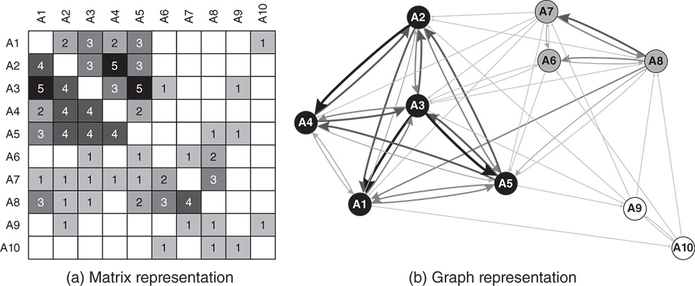
Figure 7.1 A demonstration network with ten actors.

Figure 7.2 The matrix representation of the demonstration network with erroneously reported tie values.
These types of measurement errors are hard to detect, especially the incorrectly reported values of real ties. One option for doing this is to compare the responses to an original and a reversed question. Marouf and Doreian [23] asked employees in a company about who they went to for advice and also who came to them for advice. Ideally, the reported tie value by one respondent would be confirmed by other respondent. Confirming the presence of a tie is easier than confirming its value.
An and Schramski [1] emphasized that a significant number of reported exchange ties (e.g. information, goods, or services) tend to be disputed in the reports of senders and receivers. In such disagreements, these authors argue that neither eliminating contested reports nor symmetrizing them is appropriate. Instead, they propose measuring actors credibility based on their asymmetric connections and using deterministic or stochastic methods to estimate relations between pairs of actors.
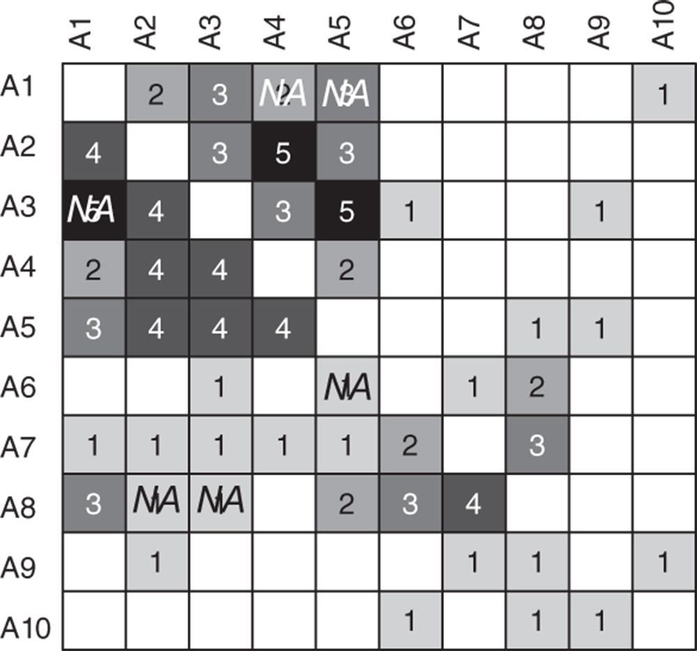
Figure 7.3 The matrix representation of the demonstration network with item non-response.
7.2.2 Item Non-Response
Item non-response occurs when one or more actors participate in a study, but provide no information on a subset of their outgoing ties. Figure 7.3 presents the demonstration network with six missing ties.
Studies of item non-response are limited. Borgatti et al. [7] stressed how absent ties “can lead to a radically different understanding of the network and misleading measurements of network indices such as centrality”. Similarly, Huisman [17] emphasized the risks of severely biased results of network analyses if missing ties are ignored.
Huisman [17] studied the impact of three imputation methods (reconstruction, hot deck,1 and preferential attachment) to estimate the mean degree, reciprocity, values of the clustering coefficient, assortativity, and inverse geodesic distances. He emphasized that, for directed networks, reconstruction was the best among the imputation methods he studied. In contrast, both preferential attachment and hot deck imputations created greater bias.2
The impacts of four treatments (reconstruction, imputations based on modal values, combination of the reconstruction and imputations based on modal values, and null tie imputations) for absent ties or item non-response on the results of blockmodeling based on structural equivalence were studied with four real networks by Žnidaršič et al. [32]. Their main conclusions were (i) the combination of reconstruction and imputations based on modal values is the best overall treatment method for absent ties, especially in networks with high reciprocity with symmetrical blockmodel structures, and (ii) for networks with low reciprocity, imputation based on modal values performed well. Null tie imputation was the worst treatment for absent ties.
7.2.3 Actor Non-Response
Actor non-response occurs where actors provide no information on any of the ties to all other members of the network. In a network with ![]() actors where
actors where ![]() actors provide no information on their outgoing tie values, the actor response rate, the “relational response rate” [19], is
actors provide no information on their outgoing tie values, the actor response rate, the “relational response rate” [19], is ![]() . With three non-respondents in the demonstration network, the relational response rate is equal to 70
. With three non-respondents in the demonstration network, the relational response rate is equal to 70![]() . Žnidaršič et al. [33,34] stress that observed information from respondents to non-respondents, their incoming ties, are still available and can be very useful.
. Žnidaršič et al. [33,34] stress that observed information from respondents to non-respondents, their incoming ties, are still available and can be very useful.
Figure 7.4 presents the demonstration network with three non-respondents (![]() ,
, ![]() , and
, and ![]() ) creating three rows of missing ties (marked by NA).
) creating three rows of missing ties (marked by NA).

Figure 7.4 The matrix representation of the demonstration network with three non-respondents.
The effects of actor non-response on direct blockmodeling based on structural equivalence have been examined in case of binary networks [33] but only for a subset of the treatments presented in Section 7.3. For valued networks, the impact of missing actors on indirect blockmodeling together with employed treatments was assessed based on simulated networks [34]. Here, we focus on actor non-response to investigate the impact of seven actor non-response treatments (presented in Section 7.3) on the results of clustering both real binary and valued networks.
7.3 Treatments of Missing Data (Due to Actor Non-Response)
Stork and Richards [30] suggested that actor non-response in network data can be treated in three different ways: (i) using a complete-case analysis, (ii) using an available-case analysis, and (iii) imputing data values. In the complete-case analysis (known also as “listwise” deletion) all non-respondents are removed from the network. The result is a smaller network with compromised network boundaries as noted by Stork and Richards. Here, we omit the complete-case approach from our simulations.3 This strategy is worthless for examining both the macro structure via blockmodeling and assessing the micro positions of all network members including non-respondents.
Seven actor non-response treatments (reconstruction, imputations of the mean values of incoming ties, imputations of the modal values of incoming ties, reconstruction and imputations based on modal values of incoming ties, imputations of the total mean, imputations of the median of the three nearest neighbors based on incoming ties, and null tie imputations) are presented in the following subsections for the small demonstration network of ten actors as presented in Figure 7.1.4 In addition to comparisons of imputed or estimated tie values, the impact of treatments on more general network characteristics is discussed.
If ![]() ,
, ![]() , and
, and ![]() refused to respond three rows of missing data will result. Table 7.1, first information line, presents some summary information about this demonstration network. First, the average outgoing tie values of these non-respondents (
refused to respond three rows of missing data will result. Table 7.1, first information line, presents some summary information about this demonstration network. First, the average outgoing tie values of these non-respondents (![]() ,
, ![]() , and
, and ![]() ) are 1.89, 1.11, and 0.44. Second, this network has 49 arcs of which 16 would be lost if the non-response was ignored. Third, the mean tie value is 2.245. Finally, its weighted density5 and weighted reciprocity6 are 1.222 and 0.691, respectively. All of these values provide a foundation for assessing the treatments of actor non-response discussed below.
) are 1.89, 1.11, and 0.44. Second, this network has 49 arcs of which 16 would be lost if the non-response was ignored. Third, the mean tie value is 2.245. Finally, its weighted density5 and weighted reciprocity6 are 1.222 and 0.691, respectively. All of these values provide a foundation for assessing the treatments of actor non-response discussed below.
Throughout this chapter we use the following terms: (i) a “whole network” is the known network, (ii) a “measured network” is obtained from the whole network by removing all outgoing ties for those actors providing no data about their ties, and (iii) a “treated network” is obtained by employing the actor non-response treatments applied to a measured network. The issue is how close the treated network is to the whole network. We turn now to consider the non-response treatments as applied to the demonstration network of Figure 7.1.
7.3.1 Reconstruction
Replacing the missing outgoing ties by their observed incoming ties could be used [17,30]. Unavailable rows of data for non-respondents are replaced by the corresponding columns for those actors. Of course, the resulting ties involving non-respondents and respondents are symmetric. For undirected networks, this is an available-case approach where the relationship between two individuals is measured by using the one report of the tie that exists in the data (see [30]). For directed networks, this imputation procedure estimates the missing tie from the incoming ties ([17]).
However, for two non-respondents, the reconstruction of ties between them cannot be done, therefore some additional imputations are required to estimate such tie values. In the simplest case, zeros are imputed. This treatment is called reconstruction in the following sections.
Table 7.1 Characteristics of the whole demonstration network and the seven treated networks
| Magnitude of changed ties in treated network according to the whole one without diagonal | Average (imputed) tie values of outgoing ties of non-respondents | Network characteristics | |||||||||||||||
| Network | 0 | 1 | 2 | 3 | A5 | A7 | A9 | Arcs | recW | densW | Mean tie value | QAP corr. | |||||
| Demonstration network | 1.89 | 1.11 | 0.44 | 49 | 0.691 | 1.222 | 2.245 | ||||||||||
| Treated networks | RE | 1 | 11 | 73 | 5 | 1.78 | 0.56 | 0.22 | 42 | 0.843 | 1.133 | 2.429 | 0.953 | ||||
| MEAN | 4 | 4 | 69 | 9 | 4 | 1.22 | 1.33 | 1.44 | 54 | 0.591 | 1.278 | 2.130 | 0.882 | ||||
| MO | 2 | 2 | 1 | 10 | 71 | 1 | 2 | 1 | 0.33 | 0.56 | 0.56 | 37 | 0.522 | 1.150 | 2.486 | 0.811 | |
| REMO | 1 | 10 | 73 | 6 | 1.78 | 0.67 | 0.33 | 44 | 0.827 | 1.156 | 2.364 | 0.952 | |||||
| TM | 3 | 2 | 1 | 74 | 10 | 1 | 1 | 1 | 59 | 0.623 | 1.178 | 1.797 | 0.878 | ||||
| kNNMedian | 11 | 74 | 3 | 2 | 1.56 | 0.67 | 0.78 | 45 | 0.660 | 1.178 | 2.356 | 0.949 | |||||
| NTI | 3 | 2 | 1 | 11 | 73 | 0 | 0 | 0 | 32 | 0.506 | 0.878 | 2.469 | 0.817 | ||||
RE, reconstruction; MEAN, imputations of the mean values of incoming ties; MO, imputations of the modal values of incoming ties; REMO, reconstruction and imputations based on modal values of incoming ties; TM, imputations of the total mean; kNNMedian, imputations of median of three nearest neighbors based on incoming ties; NTI, null tie imputations; recW, weighted reciprocity; densW, weighted density; mean tie value, mean of tie values (without zeros).

Figure 7.5 Results of seven actor non-response treatments for the demonstration network with three non-respondents. RE, reconstruction; MEAN, imputations of mean values of incoming ties; MO, imputations of modal values of incoming ties; REMO, reconstruction and modal values; TM, imputations of total mean; MEDIAN 3-NN, median of three nearest neighbors of incoming ties; NTI, null tie imputations; SED, squared Euclidean distances between the vectors of tie values of individual non-respondents and the corresponding vector of treated values.
The imputed tie values for ![]() ,
, ![]() , and
, and ![]() in the demonstration network with the reconstruction procedure are presented in the second row in Figure 7.5. Comparison of tie values with those of the whole network (first row in the body of Figure 7.5) reveals that 17 tie values were changed. The majority (12) of missing tie values were decreased and five tie values were increased (first row in Table 7.1). The weighted reciprocity of this treated network is the highest (0.843) among all treatments because it decreased the number of ties by 22
in the demonstration network with the reconstruction procedure are presented in the second row in Figure 7.5. Comparison of tie values with those of the whole network (first row in the body of Figure 7.5) reveals that 17 tie values were changed. The majority (12) of missing tie values were decreased and five tie values were increased (first row in Table 7.1). The weighted reciprocity of this treated network is the highest (0.843) among all treatments because it decreased the number of ties by 22![]() . This is not surprising. As noted above, for the ties between non-respondents (
. This is not surprising. As noted above, for the ties between non-respondents (![]() ,
, ![]() ,
, ![]() ,
, ![]() ,
, ![]() ,
, ![]() ) zeros are imputed. For
) zeros are imputed. For ![]() , the average tie value of imputed outgoing ties is 1.78, for
, the average tie value of imputed outgoing ties is 1.78, for ![]() it is 0.56, and for
it is 0.56, and for ![]() it is 0.22. The mean tie value (without zeros) is equal to 2.429, 8
it is 0.22. The mean tie value (without zeros) is equal to 2.429, 8![]() higher compared to the whole network.
higher compared to the whole network.
The right-most column of Table 7.1 shows the quadratic assignment procedure (QAP) correlation values of the treated networks with the whole network. While there is considerable variation in these values, all are significant, with ![]() values less than 0.000. However, the three highest values are noteworthy, as is discussed below.
values less than 0.000. However, the three highest values are noteworthy, as is discussed below.
7.3.2 Imputations of the Mean Values of Incoming Ties
This treatment imputes the average value of incoming ties of an actor, known as the “item mean” (imputation) [17]. For each missing outgoing tie ![]() of the non-respondent
of the non-respondent ![]() , the (rounded) mean value of all available incoming ties of actor
, the (rounded) mean value of all available incoming ties of actor ![]() is imputed.
is imputed.
As emphasized by Žnidaršič et al. [33] for binary networks, this implies (due to rounding) imputing modal values of incoming ties which led them to introduce the term “imputations based on modal value of incoming ties” for binary networks. Although, the imputations of the mean values of incoming ties and the modal values of incoming ties are the same for binary networks, the differences between them in the case of valued networks can be substantial.
The imputed tie values based on imputations of the mean value of incoming ties for three non-respondents (![]() ,
, ![]() , and
, and ![]() ) are presented in the third row in Figure 7.5. For the three non-respondents, a total of 22 tie values (equal to 1 or higher) were imputed and two 1s were set to zero. Of these, 21 tie values differed from the known true values. This is the highest number of “changed” ties compared to the whole demonstration network, suggesting serious flaws with this imputation method. The weighted reciprocity for the treated network is 0.591 and the weighted density is 1.278 (see the second row in Table 7.1), the highest among all the treated networks. The average tie values of the imputed outgoing ties are 1.22, 1.33, and 1.44 for the non-respondents
) are presented in the third row in Figure 7.5. For the three non-respondents, a total of 22 tie values (equal to 1 or higher) were imputed and two 1s were set to zero. Of these, 21 tie values differed from the known true values. This is the highest number of “changed” ties compared to the whole demonstration network, suggesting serious flaws with this imputation method. The weighted reciprocity for the treated network is 0.591 and the weighted density is 1.278 (see the second row in Table 7.1), the highest among all the treated networks. The average tie values of the imputed outgoing ties are 1.22, 1.33, and 1.44 for the non-respondents ![]() ,
, ![]() , and
, and ![]() , respectively. The values for
, respectively. The values for ![]() and
and ![]() are poor.
are poor.
7.3.3 Imputations of the Modal Values of Incoming Ties
Imputations based on the modal values of incoming ties take into account the available incoming ties of the non-respondent. For each missing outgoing tie value ![]() of actor
of actor ![]() , the modal value of values on all available incoming ties to actor
, the modal value of values on all available incoming ties to actor ![]() is imputed.7
is imputed.7
The imputed tie values using imputations of the modal values of incoming ties for three non-respondents (![]() ,
, ![]() , and
, and ![]() ) are presented in the fourth row in Figure 7.5. Multiple modal values for incoming ties to actor
) are presented in the fourth row in Figure 7.5. Multiple modal values for incoming ties to actor ![]() exist: 1 and 3. The mean value of available incoming ties is 2, meaning that the difference of mean value to both modes is equal to 1. Therefore, one of the two modes is selected randomly. In our example in Figure 7.5 and Table 7.5, 3 was randomly selected for imputed ties from non-respondents to
exist: 1 and 3. The mean value of available incoming ties is 2, meaning that the difference of mean value to both modes is equal to 1. Therefore, one of the two modes is selected randomly. In our example in Figure 7.5 and Table 7.5, 3 was randomly selected for imputed ties from non-respondents to ![]() .
.
Only five tie values were imputed. Comparisons of the treated network and the demonstration network reveal that 18 ties were changed with the majority of tie values (15) being lowered, often considerably so. The weighted reciprocity of the treated network is the second lowest (0.522) among all treatments, decreasing by 24![]() compared to the corresponding value for the whole network. The average tie values of the imputed outgoing ties are 0.33, 0.56, and 0.56 (see the third row in Table 7.1) for the non-respondents
compared to the corresponding value for the whole network. The average tie values of the imputed outgoing ties are 0.33, 0.56, and 0.56 (see the third row in Table 7.1) for the non-respondents ![]() ,
, ![]() , and
, and ![]() , respectively. All these values suggest major problems with this imputation method. Indeed, for
, respectively. All these values suggest major problems with this imputation method. Indeed, for ![]() and
and ![]() , the average of imputed tie values is the lowest among all treatments except for null tie imputations.
, the average of imputed tie values is the lowest among all treatments except for null tie imputations.
7.3.4 Reconstruction and Imputations Based on Modal Values of Incoming Ties
As noted in Section 7.3.1, reconstructing ties between non-respondents cannot be done without making additional assumptions regarding ties between the non-respondents. We combined the reconstruction procedure with imputations based on the modal values of incoming ties, although any other imputation procedure (e.g. imputations of the total mean, imputations of the mean values of incoming ties) could be used.
Comparing the treated network (fifth row in Figure 7.5) to the whole network (first row in Figure 7.5) reveals that 17 tie values were changed to values differing from the known ties. Ten tie values were decreased by 1, one tie value was decreased by 2, and six tie values were increased by 1 (fourth row in Table 7.1). The average tie values of the imputed outgoing ties are 1.78, 0.67, and 0.33 for the non-respondent ![]() ,
, ![]() , and
, and ![]() , respectively. The weighted reciprocity is 0.827, the second highest among treatments considered here being 19.7
, respectively. The weighted reciprocity is 0.827, the second highest among treatments considered here being 19.7![]() higher than for the whole network. The weighted density of the treated network compared to the whole network decreased by 5.4
higher than for the whole network. The weighted density of the treated network compared to the whole network decreased by 5.4![]() , while the mean tie value (without zeros) increased by 5.3
, while the mean tie value (without zeros) increased by 5.3![]() .
.
7.3.5 Imputations of the Total Mean
For binary networks, the average number of ties in the network is used to impute values for the missing ties. If the threshold is set to 0.5, as suggested by Huisman [17], this implies imputing zeros for the missing ties in sparse networks and ones in denser networks.
The generalization for valued networks uses the (rounded) mean of all available tie values for imputing the missing ties. When there are ![]() non-respondents in the network with
non-respondents in the network with ![]() actors, the total mean is calculated using
actors, the total mean is calculated using ![]() . For the whole network in 7.1a the average available tie value
. For the whole network in 7.1a the average available tie value ![]() . So, the value of 1 was imputed instead of missing ties in the treated network in the sixth row in Figure 7.5.
. So, the value of 1 was imputed instead of missing ties in the treated network in the sixth row in Figure 7.5.
As shown in Table 7.1, 16 tie values were changed by this imputation. The weighted density (1.178) and weighted reciprocity (0.623) both decreased compared to the whole network. The mean tie value (disregarding zeros) is 1.797 (see the fifth row in Table 7.1), the lowest among all treatments, being 20![]() lower than the corresponding value for the whole network.
lower than the corresponding value for the whole network.
7.3.6 Imputations of Median of the Three Nearest Neighbors based on Incoming Ties
The nearest-neighbor algorithm has been used widely in social surveys for estimating missing data. It was adjusted for use on network data by Žnidaršič et al. [34], who observed “the rationale for this imputation is that the non-respondents are treated individually and not as a group”. This treatment can be summarized in four steps. First, the Euclidean distances between actors are computed based on their incoming ties.8 Second, for each non-respondent the three nearest neighbors (denoted by ![]() ,
, ![]() , and
, and ![]() ) are selected using the smallest calculated Euclidean distance. Third, for each missing outgoing tie
) are selected using the smallest calculated Euclidean distance. Third, for each missing outgoing tie ![]() of non-respondent i, the median of corresponding outgoing tie values of three nearest actors (labeled
of non-respondent i, the median of corresponding outgoing tie values of three nearest actors (labeled ![]() ,
, ![]() ,
, ![]() ) is calculated. Finally, this value is imputed for the missing tie.
) is calculated. Finally, this value is imputed for the missing tie.
The imputed tie values for non-respondents ![]() ,
, ![]() , and
, and ![]() for the demonstration network are shown in the seventh row in Figure 7.5. Compared to the tie values of the whole network, 16 tie values differed from the true values. Eleven tie values were decreased by 1, three were increased by 1, and two were increased by 2 (sixth row in Table 7.1). Compared to other treatments, this is the smallest number of tie values differing from the known values, a good feature. Furthermore, the network characteristics of this treated network are closest to those of the whole network, another indication of the utility of this imputation method. For
for the demonstration network are shown in the seventh row in Figure 7.5. Compared to the tie values of the whole network, 16 tie values differed from the true values. Eleven tie values were decreased by 1, three were increased by 1, and two were increased by 2 (sixth row in Table 7.1). Compared to other treatments, this is the smallest number of tie values differing from the known values, a good feature. Furthermore, the network characteristics of this treated network are closest to those of the whole network, another indication of the utility of this imputation method. For ![]() , the average tie value on imputed outgoing ties is 1.56. For both
, the average tie value on imputed outgoing ties is 1.56. For both ![]() and
and ![]() , it is equal to 0.67 and 0.78, respectively (sixth row in Table 7.1). The weighted reciprocity and weighted density decreased by 4.5
, it is equal to 0.67 and 0.78, respectively (sixth row in Table 7.1). The weighted reciprocity and weighted density decreased by 4.5![]() and 3.6
and 3.6![]() , respectively, compared to the whole network. The mean tie value (without zeros) is equal to 2.356, also the closest to the mean tie value of the whole network.
, respectively, compared to the whole network. The mean tie value (without zeros) is equal to 2.356, also the closest to the mean tie value of the whole network.
7.3.7 Null Tie Imputations
This treatment simply imputes zeros for all missing tie values of each non-respondent. It is known as the worst treatment for obtaining blockmodel structures of both binary [33] and valued networks [34]. Although it is unlikely to be a good treatment, it is included for comparison with other treatments.
The imputed ties using null tie imputations are presented in the eighth row of Figure 7.5. A total of 17 tie values in this treated network differed for those in the whole network (seventh row of Table 7.1). Much worse, the treated network has only 32 arcs. The weighted reciprocity decreased by 26.8![]() with the weighted density decreasing by 28.2
with the weighted density decreasing by 28.2![]() compared to the whole network. Both these measures are the lowest among all the treated networks.
compared to the whole network. Both these measures are the lowest among all the treated networks.
These simple descriptive results regarding the nature of the imputed values under the seven treatments suggest that blockmodels of the different treated networks will vary greatly. This is pursued in Section 7.3.8.
7.3.8 Blockmodel Results for the Whole and Treated Networks
The basic idea in evaluating the impact of actor non-response treatments on clustering is to compare the clustering results obtained for the whole and treated networks.
There are two distinct approaches, direct and indirect (described in Section 7.4.1), to blockmodeling network data. Both aim to partition actors into clusters based on a selected equivalence. The results reported below were obtained using the indirect approach for the whole and all seven treated demonstration networks.
Table 7.2 Cluster membership of the actors the whole demonstration network and the seven treated networks
| Actor's membership in clusters based on indirect blocmodeling | |||||
| Network | Cluster 1 | Cluster 2 | Cluster 3 | ARI | |
| Demonstration network | |||||
| Treated networks | RE | 1 | |||
| MEAN | 0.378 | ||||
| MO | 0.501 | ||||
| REMO | 1 | ||||
| TM | 0.378 | ||||
| kNNMedian | 1 | ||||
| NTI | 0.501 | ||||
RE, reconstruction; MEAN, imputations of the mean values of incoming ties; MO, imputations of the modal values of incoming ties; REMO, reconstruction and imputations based on modal values of incoming ties; TM, imputations of the total mean; kNNMedian, imputations of median of three nearest neighbors based on incoming ties; NTI, null tie imputations; ARI, Adjusted Rand Index between the whole partition and the corresponding treated partition.
From the macro-structural perspective, the two partitions must be compared. The Adjusted Rand Index (ARI) is very useful for assessing the extent to which partitions coincide (or not). Its definition, based on the Rand Index [16], measures the concordance between two partitions and is corrected for chance [29], enabling comparisons of its values across different networks regarding their size and number of clusters in the underlying partition. The expected value of ARI is 0 and its maximal value is 1. General guidelines for interpreting the ARI values [29] are (i) ![]() indicates excellent agreement, (ii)
indicates excellent agreement, (ii) ![]() suggests good agreement, (iii)
suggests good agreement, (iii) ![]() indicates moderate agreement, and iv)
indicates moderate agreement, and iv) ![]() indicates poor agreement. Based on these criteria, we claim agreement between two partitions is acceptable if ARI values are above 0.8.
indicates poor agreement. Based on these criteria, we claim agreement between two partitions is acceptable if ARI values are above 0.8.
Table 7.2 shows the known blockmodel partition of the whole network and the partitions obtained, using the same blockmodeling method, for the seven treated networks. Three imputation methods lead to blockmodels identical to the known partition: reconstruction, the combination of the reconstruction and imputations based on modal values of incoming ties, and imputations using the median of the three nearest neighbors based on incoming ties. The right-hand column of Table 7.2 reports the ARI values comparing the resulting blockmodels. It takes the maximum value of 1 for these treatments. These are the three treatments whose QAP correlations are close to 1 in Table 7.1. This suggests strongly that having a significant QAP correlation for a whole and treated network is not a strong enough criterion for an acceptable imputation method. The ARI values shown for the other four imputation treatments are totally unacceptable despite the high QAP correlations between these four treated networks and the whole network. In short, blockmodels from these four treated networks are worthless.
Figure 7.5 presents, in addition to the treated tie values, the squared Euclidean distances (SED) between the vectors of tie values of individual non-respondents and the corresponding vector of treated values. For non-respondents ![]() and
and ![]() , their outgoing ties are the closest to the vector of outgoing ties treated by the median of the three nearest neighbors based on incoming ties, since the SED values are 6 and 3, respectively. For the non-respondent
, their outgoing ties are the closest to the vector of outgoing ties treated by the median of the three nearest neighbors based on incoming ties, since the SED values are 6 and 3, respectively. For the non-respondent ![]() , the original tie values, according to these SED values, are closest to the vector of tie values treated by reconstruction and null tie imputations (
, the original tie values, according to these SED values, are closest to the vector of tie values treated by reconstruction and null tie imputations (![]() ). This indicates that the median of three nearest neighbors based on incoming ties, most likely, is among the most successful treatments for estimation of missing values.
). This indicates that the median of three nearest neighbors based on incoming ties, most likely, is among the most successful treatments for estimation of missing values.
However, these results are for a network constructed solely for demonstrating some imputation treatments. We next examine some larger and real networks. We address which treatments are the more useful ones for these real networks and, perhaps more importantly, seek insights into why some treatments work better than others. Clearly, it is necessary to consider the combination of (i) the underlying structure of the networks partitioned, (ii) the nature and extent of the non-response, and (iii) the nature of the treatments for such missing data. This effort continues the research represented by the work of Žnidaršič et al. [32–34].
7.4 A Study Design Examining the Impact of Non-Response Treatments on Clustering Results
The impacts of the non-response treatments are based on clustering three distinct real networks after each has been subjected to actor non-response. We review briefly the basic distinction between indirect and direct blockmodeling in Section 7.4.1. Section 7.4.2 presents the basic design of our simulations, while in Section 7.4.3 the nature of the real networks used for our simulation study are presented.
7.4.1 Some Features of Indirect and Direct Blockmodeling
Two conceptually distinct approaches to blockmodeling are direct and indirect, as described by Batagelj et al. [4] and expanded by Doreian et al. [11]. The direct approach considers only the network data and searches for best-fitting partitions given a selected type of equivalence defined by using a set of permitted block types. A criterion function is used to evaluate the agreement between the “ideal” blocks, given a defined equivalence, and the empirically obtained blocks. For small networks, the direct approach is superior for identifying blockmodels. However, given that partitioning networks is an NP-hard problem, the direct approach is computationally burdensome, especially when networks are large.
The indirect approach (suitable for both valued and binary networks) involves two steps [11]. First, some measure of (dis)similarity between each pair of units is computed according to a selected equivalence. Second, a clustering algorithm is used to identify clusters of units. There are choices involving both the clustering algorithm used and the measures of (dis)similarity. Here, we considered only structural equivalence and used the compatible corrected Euclidean distance [4]. For clustering, we used Ward's agglomerative clustering algorithm [36] applied to these dissimilarities.
In Section 7.3.8, we described the ARI as one way of assessing the correspondence of two partitions of a network. This will be used for comparing the partitions of whole and treated real networks. We use also a second measure for binary networks: the proportion of incorrect block types in the blockmodel of a treated network compared to the blockmodel of corresponding whole network where all block types and their locations are specified. Consistent with Žnidaršič et al. [33], blockmodels of the treated networks are acceptable only if the measure, denoted by ![]() , is below 0.2.
, is below 0.2.
7.4.2 Design of the Simulation Study
The simulations were conducted by using a combination of R along with the blockmodeling package [31] and the Pajek program [2,3].
We start with a schematic outline of the simulation procedure for directed valued networks.
- For each real network, do the following:
- 1.1 Establish the partition of the whole network using indirect blockmodeling employing corrected Euclidean distance and Ward's clustering method.
- 1.2 Construct the “observed” data for a wide range for the number of non-respondents to create the measured networks. This was done by randomly selecting actors to become non-respondents and deleting all of their outgoing ties.
- 1.3 Employ each of the seven non-response data treatments (presented in Section 7.3) separately to impute values replacing missing data to create the treated networks.
- 1.4 Establish a partition of each treated network using indirect blockmodeling with the corrected Euclidean distance and Ward's clustering method.
- 1.5 Compare the partitions of the whole original and treated networks by the ARI.
Currently, the direct approach to partitioning networks is confined to binary networks. In an effort to examine the impact of actor non-response for the real networks, we modified the foregoing simulation study by establishing partitions by direct blockmodeling under structural equivalence (with the restriction of having each cluster include at least two vertices). The comparison of the partitions of the whole binary network and the treated networks was done by the ARI and the proportion of incorrect block types, ![]() .
.
7.4.3 The Real Networks Used in the Simulation Studies
We begin our analyses by using two real valued networks gathered by Marouf and Doreian [23]. These data on information and knowledge flows were collected in a Middle Eastern oil and gas company through a web survey in which all respondents were given a roster of the names of the other relevant organizational members. The questions were asked in terms of (i) the frequency with which an individual typically sought work-related information from others in the company, (ii) the frequency with which each individual gave work-related information to others, (iii) to whom did each individual typically turn for help in thinking through a new or challenging problem at work, and (iv) the frequency with which others turned to individuals for help in thinking through such new or challenging problems. The first and third relations were used to construct the reported networks. Most often, these would be the networks analyzed despite being unconfirmed. The second and fourth questions were used for constructing two confirmed networks.
In an ideal world, the relation of seeking advice and the transpose of being given advice on the same topic would correspond. In the Marouf and Doreian study [23], these relations were used to create “confirmed” networks for each of the two relations. There are two aspects to this. One concerns confirming the existence of a tie (regardless of the tie value). The second is obtaining confirmed values of the ties. The former leads to a binary network while the latter leads to a valued network. The confirmed tie regarding seeking work-related information is labeled as ![]() .
. ![]() is the label for the confirmed relation for providing help in problem solving.
is the label for the confirmed relation for providing help in problem solving.
Figure 7.6a shows the confirmed network of seeking work-related information (![]() ) with a partition according to the departments (the central administrative group, a commercial affairs group, and three drilling teams labeled A, B, and C). The confirmed network of providing help in problem solving (
) with a partition according to the departments (the central administrative group, a commercial affairs group, and three drilling teams labeled A, B, and C). The confirmed network of providing help in problem solving (![]() ) partitioned according to these five departments is presented Figure 7.6b. The shading of the squares indicates the strengths of the ties: the darker the shading, the stronger the tie. The white squares denote null ties.
) partitioned according to these five departments is presented Figure 7.6b. The shading of the squares indicates the strengths of the ties: the darker the shading, the stronger the tie. The white squares denote null ties.
The third network used in our simulations for actor non-response is a student note-borrowing network (![]() ). Data were gathered among 15 undergraduate students attending lectures [5]. Males are represented by squares and females by circles. A fitted blockmodel using structural equivalence and indirect blockmodeling produced a partition with three clusters as presented in Figure 7.7.
). Data were gathered among 15 undergraduate students attending lectures [5]. Males are represented by squares and females by circles. A fitted blockmodel using structural equivalence and indirect blockmodeling produced a partition with three clusters as presented in Figure 7.7.
Conti and Doreian [9] studied the evolution of social networks in a police academy located in a metropolitan American city. They collected network data regarding a variety of social relations at three stages of police training. One of their networks is the fourth network used in our simulations. Figure 7.8 presents a matrix representation of the “social knowledge of” relation at the second time point. The data are valued with the network labeled as ![]() . Using indirect blockmodeling yielded a partition into four clusters, which is shown in Figure 7.8.
. Using indirect blockmodeling yielded a partition into four clusters, which is shown in Figure 7.8.
Table 7.3 lists some summary details for the two valued and three binary networks (two binarized and one originally binary network). The distribution of tie values is provided along with network sizes, reciprocity (![]() ), density (
), density (![]() ), and the average tie value.
), and the average tie value.
7.5 Results
The impact of the seven non-response treatments for the real networks is presented for three types of analyses: (i) indirect blockmodeling of valued networks (in Section 7.5.1), (ii) indirect blockmodeling of binary networks (in Section 7.5.2), and (iii) direct blockmodeling of binary networks (in Section 7.5.3). In each subsection, the partition of actors in the whole networks is justified before the impacts of the actor non-response treatments are examined.
7.5.1 Indirect Blockmodeling of Real Valued Networks
According to the dendrograms presented in Figure 7.9, five clusters are appropriate when partitioning both the ![]() and
and ![]() networks using structural equivalence. Horizontal dashed lines represent cutting of the dendrogram branches. The cluster memberships of the actors are represented by grey rectangles.
networks using structural equivalence. Horizontal dashed lines represent cutting of the dendrogram branches. The cluster memberships of the actors are represented by grey rectangles.
Figure 7.10 presents matrices of ![]() and
and ![]() networks with reordered vertices according to partitions into five clusters.
networks with reordered vertices according to partitions into five clusters.

Figure 7.6 The confirmed networks for seeking work-related information and providing help in problem solving partitioned by work units.
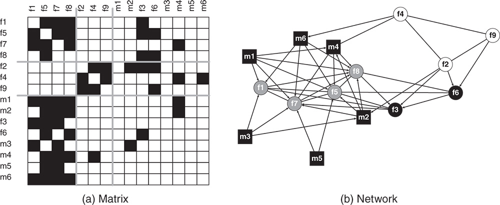
Figure 7.7 Matrix and graphical representations of the note-borrowing network with three clusters.

Figure 7.8 A valued network from a police academy with a partition obtained from indirect blockmodeling.
Table 7.3 Characteristics of three real networks and binarized version of valued ones
| Number of ties with values | Network characteristics | |||||||||
| Network | 0 | 1 | 2 | 3 | 4 | 5 | Average tie value | |||
| Valued networks | ||||||||||
| 312 | 88 | 146 | 98 | 112 | 28 | 0.822 | 1.484 | 2.527 | ||
| 433 | 96 | 103 | 56 | 68 | 28 | 0.709 | 0.981 | 2.297 | ||
| 2834 | 230 | 408 | 532 | 362 | 258 | 68 | 0.580 | 1.18 | 3.006 | |
| Binarized or binary networks | ||||||||||
| 312 | 444 | 28 | 0.973 | 0.587 | 1.000 | |||||
| 433 | 323 | 28 | 0.786 | 0.427 | 1.000 | |||||
| 169 | 56 | 15 | 0.464 | 0.267 | 1.000 | |||||
N, number of actors; recW, weighted reciprocity; densW, weighted density; mean tie value, mean of tie values (without zeros).
We now consider imposing various levels of actor non-response, treating them in seven ways and examining the consequences for the resulting blockmodels. The results of these simulations and treatments for the ![]() relation are presented in Figure 11a. The generation of missing data was repeated 28 times for networks with one missing actor (each actor was assigned to be a non-respondent) and 100 times for each combination of two or more (3, 4, 5, 6, 8, 10, 12, and 14) missing actors. Together 928 measured networks were generated and, after employment of seven treatments, we obtained 6496 treated networks. Throughout, the figures show the plots of the percentage of missing actors (ranging from 0 to 50
relation are presented in Figure 11a. The generation of missing data was repeated 28 times for networks with one missing actor (each actor was assigned to be a non-respondent) and 100 times for each combination of two or more (3, 4, 5, 6, 8, 10, 12, and 14) missing actors. Together 928 measured networks were generated and, after employment of seven treatments, we obtained 6496 treated networks. Throughout, the figures show the plots of the percentage of missing actors (ranging from 0 to 50![]() ) on the horizontal axis with the mean values of the ARI (
) on the horizontal axis with the mean values of the ARI (![]() ) on the vertical axis.
) on the vertical axis.
As expected, the trajectories for ![]() decline as the non-response gets more severe. However, the performance of the treatments differ greatly. Overall, using the median of the three nearest neighbors based on incoming ties is the superior imputation treatment. The values of
decline as the non-response gets more severe. However, the performance of the treatments differ greatly. Overall, using the median of the three nearest neighbors based on incoming ties is the superior imputation treatment. The values of ![]() are above 0.8 for 36
are above 0.8 for 36![]() non-respondents or less, indicating good agreement between the original and treated partitions. Both reconstruction treatments perform well for non-response rates of 25
non-respondents or less, indicating good agreement between the original and treated partitions. Both reconstruction treatments perform well for non-response rates of 25![]() or less. They are practically interchangeable for 21
or less. They are practically interchangeable for 21![]() non-respondents or less. This is not surprising given the relatively high value (0.822) of weighted reciprocity (
non-respondents or less. This is not surprising given the relatively high value (0.822) of weighted reciprocity (![]() ) reported in Table 7.3. For higher percentages of non-respondents, the combination of the reconstruction and imputations based on modal values performs slightly better. However, the performance of these treatments diminishes rapidly when actor non-response gets higher.
) reported in Table 7.3. For higher percentages of non-respondents, the combination of the reconstruction and imputations based on modal values performs slightly better. However, the performance of these treatments diminishes rapidly when actor non-response gets higher.
By far the worst treatment is null tie imputation. It is unacceptable for even three non-respondents (11![]() ) with
) with ![]() values below 0.8. These values diminish quickly as the non-response problem gets worse. The next two worst treatments are imputations based on the modal values of incoming ties and imputations of the total mean, since their
values below 0.8. These values diminish quickly as the non-response problem gets worse. The next two worst treatments are imputations based on the modal values of incoming ties and imputations of the total mean, since their ![]() values are below 0.8 for four (14
values are below 0.8 for four (14![]() ) and five (18
) and five (18![]() ) non-respondents, respectively. For networks having this structure, these three imputation treatments are of no real value.
) non-respondents, respectively. For networks having this structure, these three imputation treatments are of no real value.
The corresponding results for the indirect blockmodeling of the valued network ![]() are presented in Figure 7.11b. Again, the median of the three nearest neighbors based on incoming ties is the best treatment, since the values of
are presented in Figure 7.11b. Again, the median of the three nearest neighbors based on incoming ties is the best treatment, since the values of ![]() are above 0.8 for
are above 0.8 for ![]() of non-respondents. Indeed, for
of non-respondents. Indeed, for ![]() of non-respondents or less, the values of
of non-respondents or less, the values of ![]() are above 0.9, indicating excellent agreement between the two partitions. The reconstruction, the reconstruction in combination with imputations based on modal values, and imputations of the mean values of incoming ties are the next best treatments, performing satisfactorily for 36
are above 0.9, indicating excellent agreement between the two partitions. The reconstruction, the reconstruction in combination with imputations based on modal values, and imputations of the mean values of incoming ties are the next best treatments, performing satisfactorily for 36![]() of non-respondents or less. For higher percentages of non-respondents the combination of reconstruction and imputations based on modal values performs better than the other two treatments.
of non-respondents or less. For higher percentages of non-respondents the combination of reconstruction and imputations based on modal values performs better than the other two treatments.
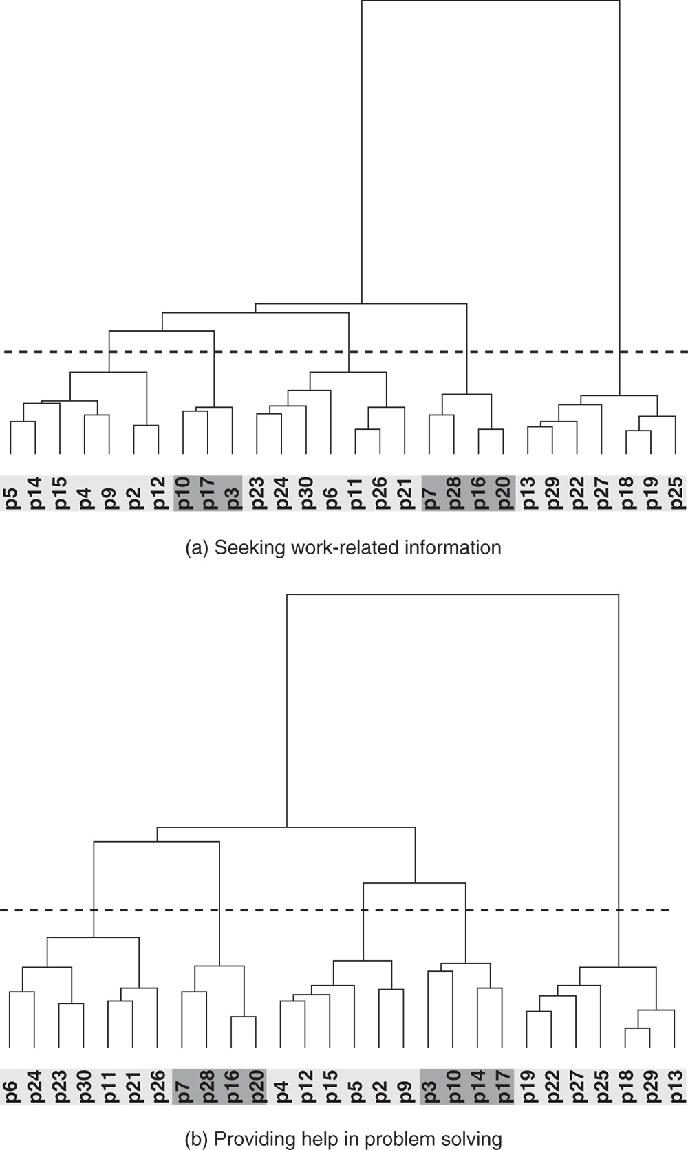
Figure 7.9 Dendrograms for the indirect blockmodeling of the confirmed (valued) networks of seeking work-related information and of providing help in problem solving.
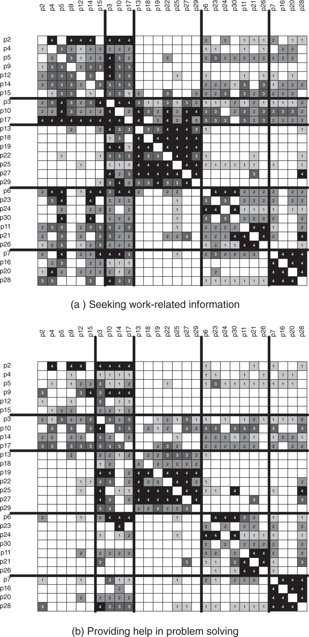
Figure 7.10 The two valued networks with partitions obtained from indirect blockmodeling.

Figure 7.11 Results of the simulation study for the indirect blockmodeling of confirmed (valued) networks of seeking work-related information and of providing help in problem solving.
Again, the three worst treatments are the null tie imputations, imputations based on the modal values of incoming ties, and imputations of the total mean, since their ![]() values are below 0.8 for five non-respondents and more, and the trajectories of their values decrease in the most extreme fashion.
values are below 0.8 for five non-respondents and more, and the trajectories of their values decrease in the most extreme fashion.
The results for the two valued networks in Figure 7.6 have some intriguing similarities and differences for the analysis of the ![]() and
and ![]() networks. The performance trajectories for the ARI measures are more sharply differentiated for the lower panel of Figure 7.11 into two groups, a reminder that the actual structure of the network matters. Yet, only one imputation method, the median of the three nearest neighbors based on incoming ties, is clearly superior. This is fully consistent with the results reported by Žnidaršič et al. [34].
networks. The performance trajectories for the ARI measures are more sharply differentiated for the lower panel of Figure 7.11 into two groups, a reminder that the actual structure of the network matters. Yet, only one imputation method, the median of the three nearest neighbors based on incoming ties, is clearly superior. This is fully consistent with the results reported by Žnidaršič et al. [34].
According to the dendrogram presented in Figure 7.12, four clusters (represented by grey rectangles according to cutting denoted by the dashed line) are appropriate when partitioning the police academy network using indirect blockmodeling.
Figure 7.8 showes a blockmodel partition with four clusters. The academy formed four squads used for para-military training, going to shooting ranges and driving training. Members of the squads identified strongly with their squads. Of some interest is that the ARI value comparing the partition in the squads and blockmodeling partition is 0.88. Conti and Doreian [9] determined, using QAP methods, that squad membership had a strong impact on relation formation at the time point for these data.
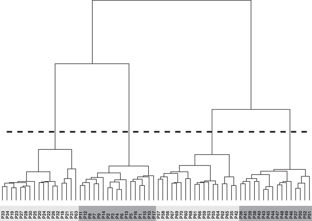
Figure 7.12 Dendrogram of the  network.

Figure 7.13 Results of the simulation study for the indirect blockmodeling of valued network from a police academy. The trajectories for reconstruction and for reconstruction and modal values are indistinguishable. The same holds for null tie imputation and imputing the mode of incoming ties.
Figure 7.13 shows the ARI trajectories for the police academy data. Yet again, the median of the three nearest neighbors outperforms all of the other imputation treatments. Indeed, for up to 30![]() of actor non-response, the ARI values are above 0.9 and, for higher levels of actor non-response, they are well above 0.8. The ARI trajectories for the two reconstruction imputation methods are virtually identical and cannot be distinguished in Figure 7.13. Up to slightly less than 30
of actor non-response, the ARI values are above 0.9 and, for higher levels of actor non-response, they are well above 0.8. The ARI trajectories for the two reconstruction imputation methods are virtually identical and cannot be distinguished in Figure 7.13. Up to slightly less than 30![]() of actor non-response, these two methods are the next best. Imputation of the total mean also performs well. Next comes imputations of the mean of incoming ties. After about 37
of actor non-response, these two methods are the next best. Imputation of the total mean also performs well. Next comes imputations of the mean of incoming ties. After about 37![]() actor non-response, the only acceptable treatment is the median of the three nearest neighbors. Imputing the mode of incoming ties and null tie imputation are virtually identical and are unacceptable when the level of actor non-response exceeds slightly less than 10
actor non-response, the only acceptable treatment is the median of the three nearest neighbors. Imputing the mode of incoming ties and null tie imputation are virtually identical and are unacceptable when the level of actor non-response exceeds slightly less than 10![]() actor non-response. They are also outperformed by all other imputation methods even for low levels of non-response.
actor non-response. They are also outperformed by all other imputation methods even for low levels of non-response.
7.5.2 Indirect Blockmodeling on Real Binary Networks
We next consider the impact of actor non-response treatment on indirect blockmodeling for three networks. The first is the student note-borrowing network (Figure 7.7). The other two networks are the binarized versions of networks ![]() and
and ![]() .
.
The dendrogram presented in Figure 7.14a reveals that actors belong to three clusters as presented in Figure 7.7, consistent with the original analysis [5]. Figure 7.14b presents the results of the actor non-response simulations with indirect blockmodeling into three clusters. The generation of missing data was repeated 15 times for networks with one missing actor (each actor was assigned to be a non-respondent), 50 times for a combinations of two non-respondents, and 100 times for combinations of three to seven missing actors. Together, 928 measured networks were generated. After employing the seven treatments, we obtained 6496 treated networks. Again, the trajectories of the mean ARI values are plotted against the percentage of missing respondents.
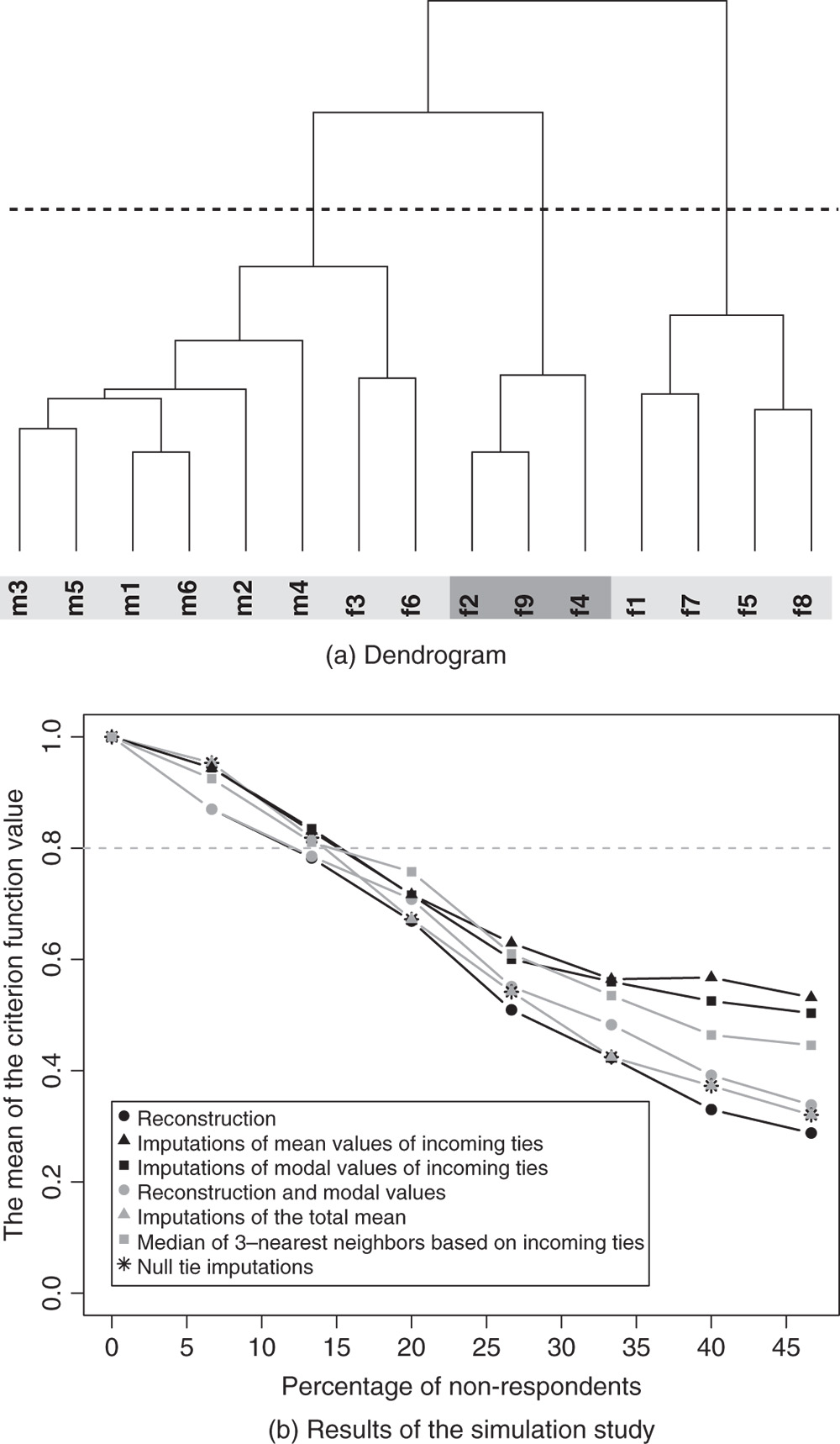
Figure 7.14 Dendrogram and results of the simulation study for the indirect blockmodeling of the note-borrowing network.
In general, the results here are less encouraging regarding the efficacy of treatments for actor non-response. Three best treatments, with interchanging rank of best performance over the whole range of non-respondents, are imputations of the mean values of incoming ties, imputations of modal values of incoming ties, and the imputation of the median of the three nearest neighbors based on incoming ties. Yet agreement between the partitions, for all treatments, is unacceptable for three (20![]() ) non-respondents or more: in this range, all
) non-respondents or more: in this range, all ![]() values are below 0.8.
values are below 0.8.
The values of ![]() for the reconstruction procedures are below those for all other treatments. We suspect the reason for reconstruction performing so badly is due to the low reciprocity (0.464) of the network. Given its low density (0.267), imputations using the total mean amounts to using null tie imputations known to be poor in general. One message is clear for networks with this structure: avoid actor non-response, a claim relevant for all networks.
for the reconstruction procedures are below those for all other treatments. We suspect the reason for reconstruction performing so badly is due to the low reciprocity (0.464) of the network. Given its low density (0.267), imputations using the total mean amounts to using null tie imputations known to be poor in general. One message is clear for networks with this structure: avoid actor non-response, a claim relevant for all networks.
As noted above, the oil company networks ![]() and
and ![]() were binarized so that each tie value of 1 or more regardless of its magnitude was set to 1. The density of the binarized
were binarized so that each tie value of 1 or more regardless of its magnitude was set to 1. The density of the binarized ![]() network is 0.587, while its reciprocity is equal to 0.973. The corresponding numbers for the binarized
network is 0.587, while its reciprocity is equal to 0.973. The corresponding numbers for the binarized ![]() network are 0.427 and 0.786.
network are 0.427 and 0.786.
The dendrogram shown in Figure 7.15a suggests five clusters are reasonable for ![]() . In contrast, a partition into four clusters is the most appropriate for
. In contrast, a partition into four clusters is the most appropriate for ![]() . This implies binarizating valued networks may be problematic, something depending on the underlying structures of networks subjected to this treatment. It seems that binarization destroys the blockmodeling structure by reducing the high variability of the original tie values. The weighted reciprocity values are higher in the binarized networks compared to the corresponding valued versions, especially for
. This implies binarizating valued networks may be problematic, something depending on the underlying structures of networks subjected to this treatment. It seems that binarization destroys the blockmodeling structure by reducing the high variability of the original tie values. The weighted reciprocity values are higher in the binarized networks compared to the corresponding valued versions, especially for ![]() (see Table 7.3). Even so, we explore the binarized networks further with regard to actor non-response.
(see Table 7.3). Even so, we explore the binarized networks further with regard to actor non-response.
Figure 7.16a presents the binarized ![]() network with the five clusters from indirect blockmodeling. Comparing the partitions based on indirect blockmodeling of the valued network (Figure 7.9a) and the binarized version of the
network with the five clusters from indirect blockmodeling. Comparing the partitions based on indirect blockmodeling of the valued network (Figure 7.9a) and the binarized version of the ![]() network (Figure 7.15a) shows they are quite different. The value of ARI confirms this since its value is 0.601. In short, the two partitions do not correspond. The four-cluster partition of the binarized
network (Figure 7.15a) shows they are quite different. The value of ARI confirms this since its value is 0.601. In short, the two partitions do not correspond. The four-cluster partition of the binarized ![]() is presented in Figure 7.16b. The ARI for partitions based on indirect blockmodeling of the valued (Figure 7.9b) and binarized (Figure 7.15b)
is presented in Figure 7.16b. The ARI for partitions based on indirect blockmodeling of the valued (Figure 7.9b) and binarized (Figure 7.15b) ![]() is 0.763, below the 0.8 threshold for being viewed as consistent partitions. Clearly, binarization of valued networks can severely change the blockmodel structure and the partition of the actors, especially if the variation in the valued tie values is large.
is 0.763, below the 0.8 threshold for being viewed as consistent partitions. Clearly, binarization of valued networks can severely change the blockmodel structure and the partition of the actors, especially if the variation in the valued tie values is large.
Figure 7.17a presents the simulation results concerning indirect blockmodeling of the ![]() network into five clusters. The imputation treatments do not fare as well as for the valued version of this network. Using the median of the three nearest neighbors performs the best for
network into five clusters. The imputation treatments do not fare as well as for the valued version of this network. Using the median of the three nearest neighbors performs the best for ![]() of non-respondents or more, although the ARI values are below the desired threshold of 0.8. This treatment is acceptable up to 11
of non-respondents or more, although the ARI values are below the desired threshold of 0.8. This treatment is acceptable up to 11![]() of non-respondents. Acceptable treatments for up to 11
of non-respondents. Acceptable treatments for up to 11![]() and
and ![]() of non-respondents are reconstruction plus modal values and simple reconstruction. All other treatment methods perform even worse, with some being unacceptable even for only two non-respondents. There is little point in comparing how badly they perform relative to each other. One reason for their wretched performance is that the binarized version of this network is almost completely symmetrical, with reciprocity equal to 0.972. If so, this suggests that only three imputation treatments have any value for highly symmetric networks.
of non-respondents are reconstruction plus modal values and simple reconstruction. All other treatment methods perform even worse, with some being unacceptable even for only two non-respondents. There is little point in comparing how badly they perform relative to each other. One reason for their wretched performance is that the binarized version of this network is almost completely symmetrical, with reciprocity equal to 0.972. If so, this suggests that only three imputation treatments have any value for highly symmetric networks.
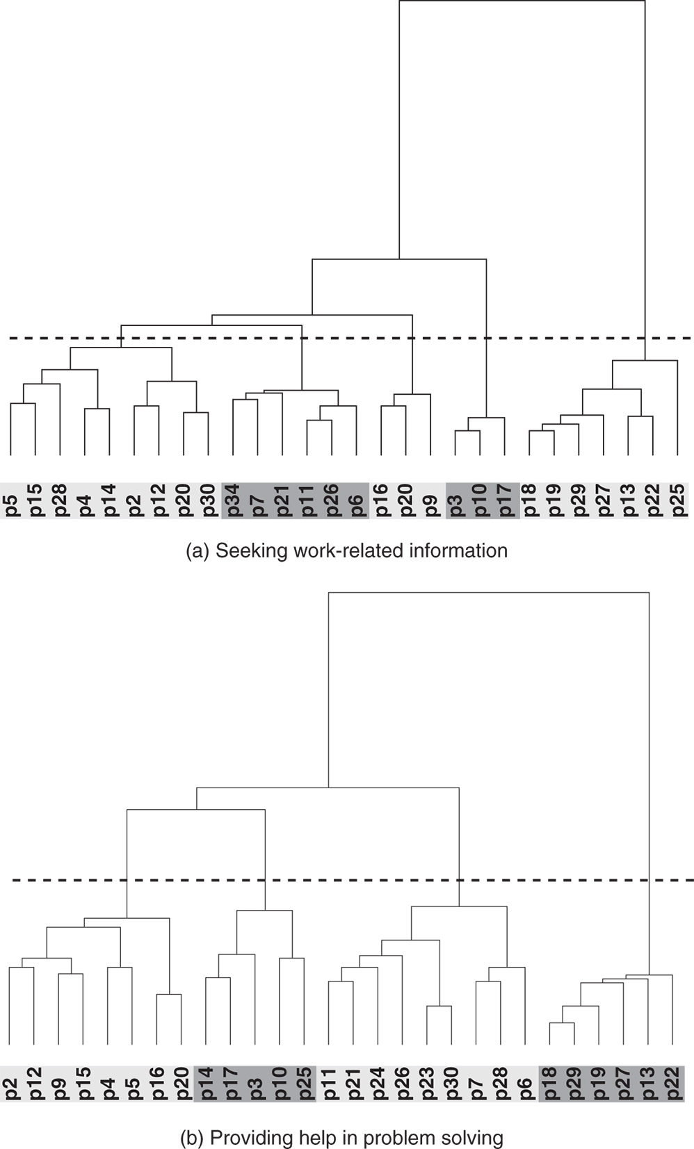
Figure 7.15 Dendrograms for the indirect blockmodeling of the binarized confirmed networks of seeking work-related information and of providing help in problem solving.

Figure 7.16 Binarized networks with partitions from indirect blockmodeling.

Figure 7.17 Results of the simulation study for the indirect blockmodeling of binarized confirmed networks of seeking work related information and of providing help in problem solving.
The impacts of actor non-response treatments using indirect blockmodeling of the ![]() network into four clusters are presented in Figure 7.17b. Again, the median of the three nearest neighbors performs the best for larger percentages of non-respondents (30
network into four clusters are presented in Figure 7.17b. Again, the median of the three nearest neighbors performs the best for larger percentages of non-respondents (30![]() or more). Up to
or more). Up to ![]() of non-respondents, its
of non-respondents, its ![]() values are above the threshold of 0.8, indicating acceptable fit between partitions. Both reconstruction procedures perform in an acceptable fashion for up to slightly more than a 20
values are above the threshold of 0.8, indicating acceptable fit between partitions. Both reconstruction procedures perform in an acceptable fashion for up to slightly more than a 20![]() level of non-response. Of the two, combinations of reconstruction and imputations of the modal values perform slightly better. All other treatments perform badly for more than 10
level of non-response. Of the two, combinations of reconstruction and imputations of the modal values perform slightly better. All other treatments perform badly for more than 10![]() of non-respondents, with
of non-respondents, with ![]() trajectories declining more sharply.
trajectories declining more sharply.
For both of the work-related networks, the median of the three nearest neighbors performs well. In these binarized networks, it performed better for the ![]() network, as it was less affected by the binarization of the two networks. Both of the treatments involving reconstruction perform well, but for lower levels of non-response compared to the superior treatment. Overall, the results reported in this section suggest there are, at most, three acceptable imputation treatments.
network, as it was less affected by the binarization of the two networks. Both of the treatments involving reconstruction perform well, but for lower levels of non-response compared to the superior treatment. Overall, the results reported in this section suggest there are, at most, three acceptable imputation treatments.
We turn to consider direct blockmodeling of these three binary networks, again using structural equivalence.
7.5.3 Direct Blockmodeling of Binary Real Networks
Under direct blockmodeling, a set of permitted block types is specified for the selected type of equivalence. For structural equivalence, only null blocks and complete blocks can be fitted to data. The value of the criterion function is the number of inconsistencies in empirical blocks compared to the ideal blocks.
The first binary network we consider is the note-borrowing network. A narrower set of treatments has already been examined for that network [33]. There, it was established that a blockmodel with three clusters delineates the macro-structure of the network (with a criterion function having 28 inconsistencies).
Continuing our general strategy, Figure 7.18a plots the value of ![]() against the percentage of actor non-response. Again, the median of the three nearest neighbors performs the best, although
against the percentage of actor non-response. Again, the median of the three nearest neighbors performs the best, although ![]() values are below 0.8 for a quarter of non-respondents and more. The second-best treatment couples reconstruction with imputations of modal values of incoming ties, but only for up to about 12
values are below 0.8 for a quarter of non-respondents and more. The second-best treatment couples reconstruction with imputations of modal values of incoming ties, but only for up to about 12![]() of non-response levels. While all of the treatment methods perform in an adequate fashion at low levels of non-response, their trajectories drop rapidly thereafter. Null tie imputation performs the worst due to the low network density (0.266), making this treatment equivalent to using the total mean. For this binarized network, reconstruction is the second worst performer, a departure from earlier results. But this is not surprising for such a non-symmetrical network (reciprocity is only 0.464).
of non-response levels. While all of the treatment methods perform in an adequate fashion at low levels of non-response, their trajectories drop rapidly thereafter. Null tie imputation performs the worst due to the low network density (0.266), making this treatment equivalent to using the total mean. For this binarized network, reconstruction is the second worst performer, a departure from earlier results. But this is not surprising for such a non-symmetrical network (reciprocity is only 0.464).
The second criterion for assessing the adequacy of identified blockmodels is the proportion of incorrect block types, ![]() . On this measure (Figure 7.18b), the differences among treatments are much smaller. Yet, the median of the three nearest neighbors remains the best treatment over a wider range of actor non-response. Up to 47
. On this measure (Figure 7.18b), the differences among treatments are much smaller. Yet, the median of the three nearest neighbors remains the best treatment over a wider range of actor non-response. Up to 47![]() of non-response, only 10
of non-response, only 10![]() of block types in the blockmodel are incorrectly identified. For lower levels of non-response the median of the three nearest neighbors does much better. The worst treatments are imputations of the total mean and null tie imputations, where for 40
of block types in the blockmodel are incorrectly identified. For lower levels of non-response the median of the three nearest neighbors does much better. The worst treatments are imputations of the total mean and null tie imputations, where for 40![]() of non-respondents, on average, 20
of non-respondents, on average, 20![]() of the block types are identified incorrectly.
of the block types are identified incorrectly.

Figure 7.18 Results of the simulation study for the direct blockmodeling of the student note-borrowing network.
Direct blockmodeling based on structural equivalence of the binarized ![]() network established a partition with five clusters. The value of the criterion function is 98.9 The binarized network of
network established a partition with five clusters. The value of the criterion function is 98.9 The binarized network of ![]() with five clusters is presented in Figure 7.19a.
with five clusters is presented in Figure 7.19a.
Figure 7.20a presents the simulation results for this network. Their most distinctive feature is the sharp separation of the trajectories of ![]() plotted against the percentage of actor non-response. Four imputation treatments are spectacularly bad for revealing position memberships of actors. Imputations of the mean value of incoming ties, imputations of the modal value of incoming ties, imputations of the total mean, and null tie imputation are unacceptable for this network. A surprise comes with the acceptable treatments. The best treatment is reconstruction with modal values. It performs well for up to about 28
plotted against the percentage of actor non-response. Four imputation treatments are spectacularly bad for revealing position memberships of actors. Imputations of the mean value of incoming ties, imputations of the modal value of incoming ties, imputations of the total mean, and null tie imputation are unacceptable for this network. A surprise comes with the acceptable treatments. The best treatment is reconstruction with modal values. It performs well for up to about 28![]() of non-respondents, although the trajectory drops sharply thereafter. The second-best treatment, up to about 18
of non-respondents, although the trajectory drops sharply thereafter. The second-best treatment, up to about 18![]() non-response levels, is the median of the three nearest neighbors based on incoming ties. Reconstruction does well up to slightly less than 20
non-response levels, is the median of the three nearest neighbors based on incoming ties. Reconstruction does well up to slightly less than 20![]() non-response and is better than using the median of the three nearest neighbors up to that level. This is due to the network being very symmetric.
non-response and is better than using the median of the three nearest neighbors up to that level. This is due to the network being very symmetric.
Regarding the identification of the correct block types, Figure 7.20b shows the best treatments are the median of the three nearest neighbors based on incoming ties and the combination of reconstruction procedure and imputations based on modal value of incoming ties. They perform very well over the entire range of non-response. Not quite as good, but still acceptable for the whole range of non-respondents, are reconstruction and imputations based on modal and median values of incoming ties.
The binarized network of ![]() with partition into four clusters is presented in Figure 7.19b. Based on this, direct blockmodeling, using structural equivalence, of the binarized
with partition into four clusters is presented in Figure 7.19b. Based on this, direct blockmodeling, using structural equivalence, of the binarized ![]() network was performed with four clusters as the dendrogram in Figure 7.15b suggests four clusters. The value of the criterion function for this partition is 143.
network was performed with four clusters as the dendrogram in Figure 7.15b suggests four clusters. The value of the criterion function for this partition is 143.
Figure 7.21b reveals, as for the binarized version of the ![]() , that four treatments, imputations of the mean and modal values of incoming ties, imputations of the total mean, and null tie imputations, perform poorly in revealing position memberships. For 21
, that four treatments, imputations of the mean and modal values of incoming ties, imputations of the total mean, and null tie imputations, perform poorly in revealing position memberships. For 21![]() of non-respondents or less both reconstruction procedures perform well. Again, using the median of the three nearest neighbors based on incoming ties is better than both reconstruction procedures being acceptable up to 35
of non-respondents or less both reconstruction procedures perform well. Again, using the median of the three nearest neighbors based on incoming ties is better than both reconstruction procedures being acceptable up to 35![]() non-respondents.
non-respondents.
In terms of ![]() values in Figure 7.21b, the best treatment is reconstruction combined with using modal values of incoming ties. Even for 50
values in Figure 7.21b, the best treatment is reconstruction combined with using modal values of incoming ties. Even for 50![]() of non-respondents values of
of non-respondents values of ![]() are around 0.1. Using the median of the three nearest neighbors based on incoming ties is acceptable also across the whole range of non-respondents. Null tie imputations and imputations of the total mean were unable to identify the macro structure of the network for 18
are around 0.1. Using the median of the three nearest neighbors based on incoming ties is acceptable also across the whole range of non-respondents. Null tie imputations and imputations of the total mean were unable to identify the macro structure of the network for 18![]() of non-respondents or more.
of non-respondents or more.

Figure 7.19 Networks with partitions from direct blockmodeling based on structural equivalence.

Figure 7.20 Results of the simulation study for the direct blockmodeling of the binarized confirmed network of seeking work-related information.
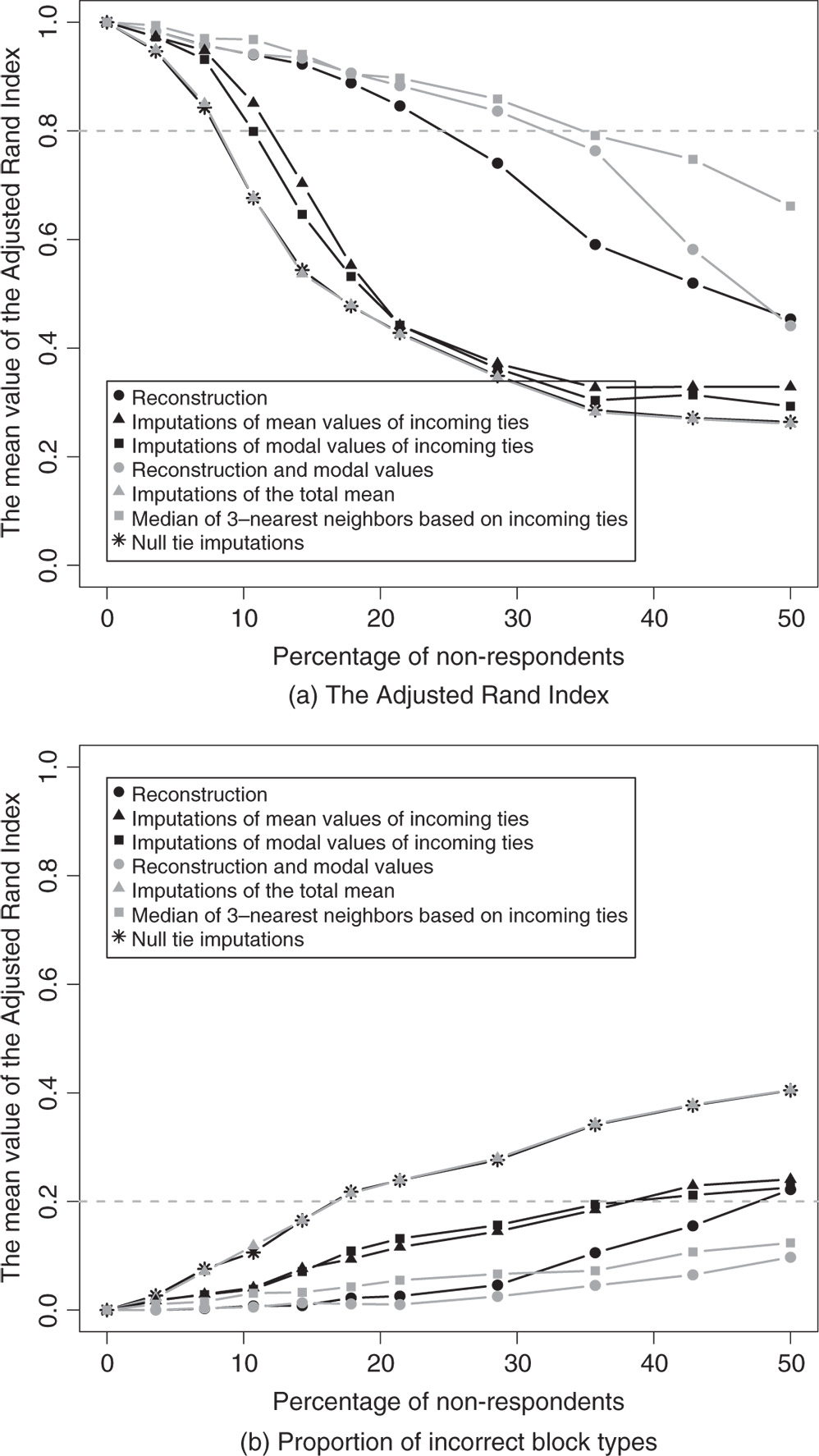
Figure 7.21 Results for the direct blockmodeling of the binarized confirmed network of providing help in problem solving.
Table 7.4 Summary of impact of actor non-response treatments on clustering
 |
RE, reconstruction; MEAN, imputations of mean values of incoming ties; MO, imputations of modal values of incoming ties; REMO, reconstruction and modal values; TM, imputations of total mean; MEDIAN 3-NN, median of three nearest neighbors based on incoming ties; NTI, null tie imputations.
7.6 Conclusions
The results from the simulations are complex. Table 7.4 provides a summary for all the studied networks and clustering procedures. For each network used in clustering, the performance of actor non-response treatments based on both the ARI (![]() ) and the proportion of incorrect block types (
) and the proportion of incorrect block types (![]() ) is presented by different shades. Bad performances are denoted by white, moderate performances by grey, and good performances by black. We note the row for the median of the three nearest neighbors, which performed well for all but one of the 12 networks examined. Below the table, weighted reciprocity is provided since the selection of the best treatment depends of the level of the symmetry and/or correspondence of tie values.
) is presented by different shades. Bad performances are denoted by white, moderate performances by grey, and good performances by black. We note the row for the median of the three nearest neighbors, which performed well for all but one of the 12 networks examined. Below the table, weighted reciprocity is provided since the selection of the best treatment depends of the level of the symmetry and/or correspondence of tie values.
Based on the results and the summary given in Table 7.4, together with the results of extensive simulation studies on three network models (cohesive subgroups, core periphery, and hierarchical model) presented by Žnidaršič et al. [34], the following recommendations can be given:
- Never disregard the non-respondents of the network. Ignoring incoming ties is an absurd strategy despite it being a frequent response to the presence of actor non-response. Doing so borders on irresponsibilty.
- Use the best possible imputation method for missing data.
- Regardless of the hypothesized blockmodel structure, the clustering procedure employed, and the level of reciprocity the most preferable actor non-response treatment is using the median of the
 nearest neighbors based on incoming ties.
 - We recommend strongly the inclusion of this imputation method for treating actor non-response and plead for its inclusion in all social network analytic packages.
- The reconstruction procedure combined with imputations based on modal values performs well, especially if a network is highly symmetrical.
- For direct blockmodeling of binarized networks, the macro structure is more stable than micro-level memberships for non-respondents in clusters.
- However, the binarization of the valued network can severely change the underlying blockmodel structure, especially when the variability of tie values is high. We claim this data analytic strategy must be avoided when partitioning networks.
The main limitation of this study is the small set of relatively small real-world networks we examined, despite the police academy data being the largest network we considered. Even so, if these results are combined with similar conclusions drawn by Žnidaršič et al. [34], the above conclusions must be emphasized. Clearly, the structure of the empirical network has great relevance for assessing the consequences of having measurement errors [34]. Using both real and completely simulated networks is, and will continue to be, useful in this effort. Actor non-response is eminently treatable but other missing data problems remain. The impact of item non-response on the results of network partitioning may be more consequential, as it is harder to detect and treat. Even more crucial is an effort to determine the influence of measurement errors in the form of misreported tie strengths of valued networks for partitioning outcomes.
Acknowledgements
This work was supported in part by the Slovenian Research Agency (research program P5-0168) and by the Russian Academic Excellence Project ‘5-100’.
References
- 1. W. An and S. Schramski. Analysis of contested reports in exchange networks based on actors' credibility. Social Networks, 40:25–33, 2015.
- 2. V. Batagelj and A. Mrvar. Pajek 5.01. 1996-2017. URL http://mrvar.fdv.uni-lj.si/pajek/. (February 1, 2017).
- 3. V. Batagelj and A. Mrvar. Pajek and Pajek-XXL, Program for Analysis and Visualization of Large Networks, Reference Manual, List of commands with short explanation, version 5.01. 1996-2017. URL mrvar.fdv.uni-lj.si/pajek/pajekman.pdf.
- 4. V. Batagelj, A. Ferligoj, and P. Doreian. Direct and indirect methods for structural equivalence. Social Networks, 14(1-2):63–90, 1992.
- 5. V. Batagelj, A. Mrvar, A. Ferligoj, and P. Doreian. Generalized blockmodeling with Pajek. Metodološki Zvezki, 1:455–467, 2004.
- 6. D. C. Bell, B. Belli-McQueen, and A. Haider. Partner naming and forgetting: Recall of network members. Social Networks, 29(2):279–299, 2007.
- 7. S. P. Borgatti, K. M. Carley, and D. Krackhardt. On the robustness of centrality measures under conditions of imperfect data. Social Networks, 28(2):124–136, 2006.
- 8. D. D. Brewer and C. M. Webster. Forgetting of friends and its effects on measuring friendship networks. Social Networks, 21(4):361–373, 2000.
- 9. N. Conti and P. Doreian. Social engineering and race in a police academy. Social Networks, 32(1):30–43, 2010.
- 10. P. Doreian and K. L. Woodard. Defining and locating cores and boundaries of social networks. Social Networks, 16(4):267–293, 1994.
- 11. P. Doreian, V. Batagelj, and A. Ferligoj. Generalized Blockmodeling. Cambridge University Press, New York, 2005.
- 12. A. Ferligoj and V. Hlebec. Evaluation of social network measurement instruments. Social Networks, 21(2):111–130, 1999.
- 13. V. Hlebec. Recall versus recognition: Comparison of the two alternative procedures for collecting social network data. Metodološki Zvezki, 9: 121–128, 1993.
- 14. V. Hlebec. Meta-analiza zanesljivosti anketnega merjenja socialne opore v popolnih omrežjih. Teorija in Praksa, 38:63–76, 2001.
- 15. P. W. Holland and S. Leinhardt. The structural implications of measurement error in sociometry. Journal of Mathematical Sociology, 3 (1):85–11, 1973.
- 16. L. Hubert and P. Arabie. Comparing Partitions. Journal of Classification, 2:193–218, 1985.
- 17. M. Huisman. Effects of missing data in social networks. Journal of Social Structure, 10(1), 2009.
- 18. M. Huisman and C. Steglich. Treatment of non-response in longitudinal network studies. Social Networks, 30(4):297–308, 2008.
- 19. D. Knoke and S. Yang. Social networks analysis. Sage Publications, Los Angeles, 2nd edition, 2008.
- 20. J. H. Koskinen, G. L. Robins, P. Wang, and P. E. Pattison. Bayesian analysis for partially observed network data, missing ties, attributes and actors. Social Networks, 35(4):514–527, 2013.
- 21. G. Kossinets. Effects of missing data in social networks. Social Networks, 28(3):247–268, 2006.
- 22. E. Laumann, P. Marsden, and D. Prensky. The boundary specification problem in network analysis. In R. Burt and M. Minor, editors, Applied Network Analysis: A Methodological Introduction, pages 18–34. Sage Publications, London, 1983.
- 23. L. Marouf and P. Doreian. Understanding information and knowledge flows as network processes in an oil company. Journal of Information and Knowledge Management, 9(2):105–118, 2010.
- 24. G. Robins, P. Pattison, and J. Woolcock. Missing data in networks: exponential random graph (p*) models for networks with non-respondents. Social Networks, 26(3):257–283, 2004.
- 25. J. Scott. Social Network Analysis. SAGE, London, 3rd edition, 2013.
- 26. J. A. Smith and J. Moody. Structural effects of network sampling coverage I: Nodes missing at random. Social Networks, 35(4):652–668, 2013.
- 27. J. A. Smith, J. Moody, and J. H. Morgan. Network sampling coverage II: The effect of non-random missing data on network measurement. Social Networks, 48:78–99, 2017.
- 28. T. Squartini, F. Picciolo, F. Ruzzenenti, and D. Garlaschelli. Reciprocity of weighted networks. Scientific Reports, 3, 2729, 2013.
- 29. D. Steinley. Properties of the Hubert-Arabie Adjusted Rand Index. Psychological Methods, 9(3):386–396, 2004.
- 30. D. Stork and W. D. Richards. Nonrespondents in communication network studies: problems and possibilities. Group and Organization Management, 17:193–209, 1992.
- 31. A. Žiberna. Blockmodeling 0.1.8: An R package for generalized and classical blockmodeling of valued networks, 2010.
- 32. A. Žnidaršič, P. Doreian, and A. Ferligoj. Absent ties in social networks, their treatments, and blockmodeling outcomes. Metodološki Zvezki, 9: 119–138, 2012.
- 33. A. Žnidaršič, A. Ferligoj, and P. Doreian. Non-response in social networks: the impact of different non-response treatments on the stability of blockmodels. Social Networks, 34:438–450, 2012.
- 34. A. Žnidaršič, A. Ferligoj, and P. Doreian. Actor non-response in valued social networks: The impact of different non-response treatments on the stability of blockmodels. Social Networks, 34:46–56, 2017.
- 35. C. Wang, C. T. Butts, J. R. Hipp, R. Jose, and C. M. Lakon. Multiple imputation for missing edge data: A predictive evaluation method with application to add health. Social Networks, 45:89–98, 2016.
- 36. J. Ward, Joe. H. Hierarchical grouping to optimize an objective function. Journal of the American Statistical Association, 58:236–244, 1963.
- 37. S. Wasserman and K. Faust. Social Network Analysis: Methods and Applications. Cambridge University Press, Cambridge, 2nd edition, 1998.
Notes
- 1 Both categorical attributes and structural properties are used to find a completely observed “donor” actor by minimizing the absolute differences between an actor with incomplete data and the donor actor. The donor actor is used to replace the missing ties (or missing actors in case of actor non-response).
- 2 Also, for item non-response, the hot deck method was unable to find donor actors to replace the missing ties if the proportion of missing ties was large.
- 3 Some results on how deletion of actors severely changes the network characteristics are provided in [7,18,26,27].
- 4 There exist other approaches to missing network data in the context of exponential random graph (
 ) models (e.g. [20,24,35]) which are not considered here.
 - 5 Density describes the general level of linkage among the actors [37] in a network. For a directed binary network with
 actors, it is defined as the number of arcs (
 ) divided by the number of all possible arcs in a network (
 ). Scott [25] noted a lack of agreement on how density should be measured in valued graphs. Here, we use a simple extension of binary density and use the average of tie values:
(7.1)
). Scott [25] noted a lack of agreement on how density should be measured in valued graphs. Here, we use a simple extension of binary density and use the average of tie values:
(7.1)
where
 is the value of the arc from actor
  to actor
  and
and  is the number of actors in the network. This weighted density measures the average tie strength.
 - 6 For valued networks, computing reciprocity for dyads is complicated. Of course, the difference between tie values in a dyad must be considered. However, the distribution of strengths has to be taken into account as well. Weighted reciprocity (
 ) is defined as [28]:
(7.2)
) is defined as [28]:
(7.2)
where
 is the value of the tie from actor
  to
to  . The upper bound of
  is 1 when all tie values are symmetrical in their values. In the case of binary networks the above definition corresponds to the definition provided in [17]:
  , where
  is number of edges and
  the number of arcs.
 - 7 If multiple modal values exist, the one closest to the average value of incoming ties is imputed.
- 8 In our simulations, we assumed that loops are not allowed in the networks, therefore diagonal values were not taken into account when calculating distances. In addition, the standard Euclidean distance measure is “corrected” in a way that the sum is scaled up proportionally to the number of columns used (according to function dist in R).
- 9 For the partition into four clusters, the criterion function had a value of 114. Worse, there were two equally well-fitting partitions. Using six clusters, the value of the criterion function dropped to 92 but, again, there were two equally well-fitting partitions. It is well known that the value of the criterion function for structural equivalence decreases monotonically with the number of clusters. Given the other partitions of this network, using more clusters seems unadvisable. Hence our choice to work with five clusters.