
Chapter 14
The Fundamentals of Using SQL
IN THIS CHAPTER
- Understanding basic SQL
- Getting fancy with advanced SQL
- Using SQL-specific queries
Structured Query Language (SQL) is the language that relational database management systems (such as Access) use to perform their various tasks. In order to tell Access to perform any kind of query, you have to convey your instructions in SQL. Don't panic—the truth is, you've already been building and using SQL statements, even if you didn't realize it.
In this chapter, you'll discover the role that SQL plays in your dealings with Access and learn how to understand the SQL statements generated when building queries. You'll also explore some of the advanced actions you can take with SQL statements, allowing you to accomplish actions that go beyond the Access user interface. The basics you learn here will lay the foundation for your ability to perform the advanced techniques you'll encounter throughout the rest of this book.
Understanding Basic SQL
A major reason your exposure to SQL is limited is that Access is more user friendly than most people give it credit for being. The fact is, Access performs a majority of its actions in user-friendly environments that hide the real grunt work that goes on behind the scenes.
For a demonstration of this, build in Design view the query you see in Figure 14.1. In this relatively simple query, you're asking for the sum of revenue by period.
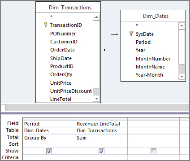
Figure 14.1 Build this relatively simple query in Design view.
Next, select the Design tab on the Ribbon and choose View ![]() SQL View. Access switches from Design view to the view you see in Figure 14.2.
SQL View. Access switches from Design view to the view you see in Figure 14.2.

Figure 14.2 You can get to SQL view by selecting View ![]() SQL View.
SQL View.
As you can see in Figure 14.2, while you were busy designing your query in Design view, Access was diligently creating the SQL statement that allows the query to run. This example shows that with the user-friendly interface provided by Access, you don't necessarily need to know the SQL behind each query. The question now becomes: If you can run queries just fine without knowing SQL, why bother to learn it?
Admittedly, the convenient query interface provided by Access does make it a bit tempting to go through life not really understanding SQL. However, if you want to harness the real power of data analysis with Access, you need to understand the fundamentals of SQL.
The SELECT statement
The SELECT statement, the cornerstone of SQL, enables you to retrieve records from a dataset. The basic syntax of a SELECT statement is as follows:
SELECT column_name(s)
FROM table_name
The SELECT statement is always used with a FROM clause. The FROM clause identifies the table(s) that make up the source for the data.
Try this: Start a new query in Design view. Close the Show Table dialog box (if it's open), select the Design tab on the Ribbon, and choose View ![]() SQL View. In SQL view, type in the
SQL View. In SQL view, type in the SELECT statement shown in Figure 14.3, and then run the query by selecting Run on the Design tab of the Ribbon.

Figure 14.3 A basic SELECT statement in SQL view.
Congratulations! You've just written your first query manually.
Selecting specific columns
You can retrieve specific columns from your dataset by explicitly defining the columns in your SELECT statement, as follows:
SELECT AccountManagerID, FullName,[Email Address]
FROM Dim_AccountManagersSelecting all columns
Using the wildcard (*) allows you to select all columns from a dataset without having to define every column explicitly.
SELECT * FROM Dim_AccountManagersThe WHERE clause
You can use the WHERE clause in a SELECT statement to filter your dataset and conditionally select specific records. The WHERE clause is always used in combination with an operator such as: = (equal), <> (not equal), > (greater than), < (less than), >= (greater than or equal to), <= (less than or equal to), or BETWEEN (within general range).
The following SQL statement retrieves only those employees whose last name is Winston:
SELECT AccountManagerID, [Last Name], [First Name]
FROM Dim_AccountManagers
WHERE [Last Name] = "Winston"
And this SQL statement retrieves only those employees whose hire date is later than May 16, 2012:
SELECT AccountManagerID, [Last Name], [First Name]
FROM Dim_AccountManagers
WHERE HireDate > #5/16/2012#Making sense of joins
You'll often need to build queries that require that two or more related tables be joined to achieve the desired results. For example, you may want to join an employee table to a transaction table in order to create a report that contains both transaction details and information on the employees who logged those transactions. The type of join used will determine the records that will be output.
Inner joins
An inner join operation tells Access to select only those records from both tables that have matching values. Records with values in the joined field that do not appear in both tables are omitted from the query results.
The following SQL statement selects only those records in which the employee numbers in the AccountManagerID field are in both the Dim_AccountManagers table and the Dim_Territory table.
SELECT Region, Market,
Dim_AccountManagers.AccountManagerID, FullName
FROM Dim_AccountManagers INNER JOIN Dim_Territory ON
Dim_AccountManagers.AccountManagerID =
Dim_Territory.AccountManagerID
Outer joins
An outer join operation tells Access to select all the records from one table and only the records from a second table with matching values in the joined field. There are two types of outer joins: left joins and right joins.
A left join operation (sometimes called an outer left join) tells Access to select all the records from the first table regardless of matching and only those records from the second table that have matching values in the joined field.
This SQL statement selects all records from the Dim_AccountManagers table and only those records in the Dim_Territory table where values for the AccountManagerID field exist in the Dim_AccountManagers table.
SELECT Region, Market,
Dim_AccountManagers.AccountManagerID, FullName
FROM Dim_AccountManagers LEFT JOIN Dim_Territory ON
Dim_AccountManagers.AccountManagerID =
Dim_Territory.AccountManagerID
A right join operation (sometimes called an outer right join) tells Access to select all the records from the second table, regardless of matching, and only those records from the first table that have matching values in the joined field.
This SQL statement selects all records from the Dim_Territory table and only those records in the Dim_AccountManagers table where values for the AccountManagerID field exist in the Dim_Territory table.
SELECT Region, Market,
Dim_AccountManagers.AccountManagerID, FullName
FROM Dim_AccountManagers RIGHT JOIN Dim_Territory ON
Dim_AccountManagers.AccountManagerID =
Dim_Territory.AccountManagerIDGetting Fancy with Advanced SQL Statements
You'll soon realize that the SQL language is quite versatile, allowing you to go far beyond basic SELECT, FROM, and WHERE statements. In this section, you'll explore some of the advanced actions you can accomplish with SQL.
Expanding your search with the Like operator
By itself, the Like operator is no different from the equal (=) operator. For instance, these two SQL statements will return the same number of records:
SELECT AccountManagerID, [Last Name], [First Name]
FROM Dim_AccountManagers
WHERE [Last Name] = "Winston"
SELECT AccountManagerID, [Last Name], [First Name]
FROM Dim_AccountManagers
WHERE [Last Name] Like "Winston"
The Like operator is typically used with wildcard characters to expand the scope of your search to include any record that matches a pattern. The wildcard characters that are valid in Access are as follows:
- *: The asterisk represents any number and type characters.
- ?: The question mark represents any single character.
- #: The pound sign represents any single digit.
- []: The brackets allow you to pass a single character or an array of characters to the
Likeoperator. Any values matching the character values within the brackets will be included in the results. - [!]: The brackets with an embedded exclamation point allow you to pass a single character or an array of characters to the
Likeoperator. Any values matching the character values following the exclamation point will be excluded from the results.
Listed in Table 14.1 are some example SQL statements that use the Like operator to select different records from the same table column.
Table 14.1 Selection Methods Using the Like Operator
| Wildcard Character(s) Used | SQL Statement Example | Result |
* |
SELECT Field1FROM Table1WHERE Field1 Like "A*" |
Selects all records where Field1 starts with the letter A |
* |
SELECT Field1FROM Table1WHERE Field1 Like "*A*" |
Selects all records where Field1 includes the letter A |
? |
SELECT Field1FROM Table1WHERE Field1 Like "???" |
Selects all records where the length of Field1 is three characters long |
? |
SELECT Field1FROM Table1WHERE Field1 Like "B??" |
Selects all records where Field1 is a three-letter string that starts with B |
# |
SELECT Field1FROM Table1WHERE Field1 Like "###" |
Selects all records where Field1 is a number that is exactly three digits long |
# |
SELECT Field1FROM Table1WHERE Field1 Like "A#A" |
Selects all records where the value in Field1 is a three-character value that starts with A, contains one digit, and ends with A |
#, * |
SELECT Field1FROM Table1WHERE Field1 Like "A#*" |
Selects all records where Field1 begins with A and any digit |
[], * |
SELECT Field1FROM Table1WHERE Field1 Like "*[$%!*/]*" |
Selects all records where Field1 includes any one of the special characters shown in the SQL statement |
[!], * |
SELECT Field1FROM Table1WHERE Field1 Like "*[!a-z]*" |
Selects all records where the value of Field1 is not a text value, but a number value or special character such as the @ symbol |
[!], * |
SELECT Field1FROM Table1WHERE Field1 Like "*[!0-9]*" |
Selects all records where the value of Field1 is not a number value, but a text value or special character such as the @ symbol |
Selecting unique values and rows without grouping
The DISTINCT predicate enables you to retrieve only unique values from the selected fields in your dataset. For example, the following SQL statement will select only unique job titles from the Dim_AccountManagers table, resulting in six records:
SELECT DISTINCT AccountManagerID
FROM Dim_AccountManagers
If your SQL statement selects more than one field, the combination of values from all fields must be unique for a given record to be included in the results.
If you require that the entire row be unique, you could use the DISTINCTROW predicate. The DISTINCTROW predicate enables you to retrieve only those records for which the entire row is unique. That is to say, the combination of all values in the selected fields does not match any other record in the returned dataset. You would use the DISTINCTROW predicate just as you would in a SELECT DISTINCT clause.
SELECT DISTINCTROW AccountManagerID
FROM Dim_AccountManagers
Grouping and aggregating with the GROUP BY clause
The GROUP BY clause makes it possible to aggregate records in your dataset by column values. When you create an aggregate query in Design view, you're essentially using the GROUP BY clause. The following SQL statement will group the Market field and give you the count of states in each market:
SELECT Market, Count(State)
FROM Dim_Territory
GROUP BY Market
When you're using the GROUP BY clause, any WHERE clause included in the query is evaluated before aggregation occurs. However, you may have scenarios when you need to apply a WHERE condition after the grouping is applied. In these cases, you can use the HAVING clause.
For instance, this SQL statement will group the records where the value in the Market field is Dallas, and then only return those customer records where the sum of Revenue is less than 100. Again, the grouping is done before checking if the sum of Revenue is less than 100.
SELECT Customer_Name, Sum(Revenue) AS Sales
FROM PvTblFeed
Where Market = "Dallas"
GROUP BY Customer_Name
HAVING (Sum(Revenue)<100)
Setting the sort order with the ORDER BY clause
The ORDER BY clause enables you to sort data by a specified field. The default sort order is ascending; therefore, sorting your fields in ascending order requires no explicit instruction. The following SQL statement will sort the resulting records by Last Name ascending and then First Name ascending:
SELECT AccountManagerID, [Last Name], [First Name]
FROM Dim_AccountManagers
ORDER BY [Last Name], [First Name]
To sort in descending order, you must use the DESC reserved word after each column you want sorted in descending order. The following SQL statement will sort the resulting records by Last Name descending and then First Name ascending:
SELECT AccountManagerID, [Last Name], [First Name]
FROM Dim_AccountManagers
ORDER BY [Last Name] DESC, [First Name]
Creating aliases with the AS clause
The AS clause enables you to assign aliases to your columns and tables. There are generally two reasons you would want to use aliases: Either you want to make column or table names shorter and easier to read, or you're working with multiple instances of the same table and you need a way to refer to one instance or the other.
Creating a column alias
The following SQL statement will group the Market field and give you the count of states in each market. In addition, the alias State Count has been given to the column containing the count of states by including the AS clause.
SELECT Market, Count(State) AS [State Count]
FROM Dim_Territory
GROUP BY Market
HAVING Market = "Dallas"
Creating a table alias
This SQL statement gives the Dim_AccountManagers the alias “MyTable.”
SELECT AccountManagerID, [Last Name], [First Name]
FROM Dim_AccountManagers AS MyTable
Showing only the SELECT TOP or SELECT TOP PERCENT
When you run a SELECT query, you're retrieving all records that meet your definitions and criteria. When you run the SELECT TOP statement, or a top values query, you're telling Access to filter your returned dataset to show only a specific number of records.
Top values queries explained
To get a clear understanding of what the SELECT TOP statement does, build the aggregate query shown in Figure 14.4.

Figure 14.4 Build this aggregate query in Design view. Take note that the query is sorted descending on the Sum of LineTotal.
On the Query Tools Design tab, click the Property Sheet command. This will activate the Property Sheet dialog box shown in Figure 14.5. Alternatively, you can use the F4 key on your keyboard to activate the Property Sheet dialog box.
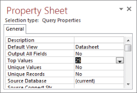
Figure 14.5 Change the Top Values property to 25.
In the Property Sheet dialog box, change the Top Values property to 25.
As you can see in Figure 14.6, after you run this query, only the customers who fall into the top 25 by sum of revenue are returned. If you want the bottom 25 customers, simply change the sort order of the LineTotal field to Ascending.
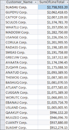
Figure 14.6 Running the query will give you the top 25 customers by revenue.
The SELECT TOP statement
The SELECT TOP statement is easy to spot. This is the same query used to run the results in Figure 14.6:
SELECT TOP 25 Customer_Name, Sum(LineTotal) AS SumOfLineTotal
FROM Dim_Customers INNER JOIN Dim_Transactions ON
Dim_Customers.CustomerID = Dim_Transactions.CustomerID
GROUP BY Customer_Name
ORDER BY Sum(LineTotal) DESC
Bear in mind that you don't have to be working with totals or currency to use a top values query. In the following SQL statement, you're returning the ten account managers that have the earliest hire date in the company, effectively producing a seniority report:
SELECT Top 10 AccountManagerID, [Last Name], [First Name]
FROM Dim_AccountManagers
ORDER BY HireDate ASCThe SELECT TOP PERCENT statement
The SELECT TOP PERCENT statement works in exactly the same way as SELECT TOP except the records returned in a SELECT TOP PERCENT statement represent the nth percent of total records rather than the nth number of records. For example, the following SQL statement will return the top 25 percent of records by revenue:
SELECT TOP 25 PERCENT Customer_Name, Sum(LineTotal) AS SumOfLineTotal
FROM Dim_Customers INNER JOIN Dim_Transactions ON
Dim_Customers.CustomerID = Dim_Transactions.CustomerID
GROUP BY Customer_Name
ORDER BY Sum(LineTotal) DESCPerforming action queries via SQL statements
You may not have thought about it before, but when you build an action query, you're building a SQL statement that is specific to that action. These SQL statements make it possible for you to go beyond just selecting records.
Make-table queries translated
Make-table queries use the SELECT…INTO statement to make a hard-coded table that contains the results of your query. The following example first selects account manager number, last name, and first name; and then it creates a new table called Employees:
SELECT AccountManagerID, [Last Name], [First Name] INTO Employees
FROM Dim_AccountManagers
Append queries translated
Append queries use the INSERT INTO statement to insert new rows into a specified table. The following example inserts new rows into the Employees table from the Dim_AccountManagers table:
INSERT INTO Employees (AccountManagerID, [Last Name], [First Name])
SELECT AccountManagerID, [Last Name], [First Name]
FROM Dim_AccountManagers
Update queries translated
Update queries use the UPDATE statement in conjunction with SET in order to modify the data in a dataset. This example updates the List_Price field in the Dim_Products table to increase prices by 10 percent:
UPDATE Dim_Products SET List_Price = [List_Price]*1.1Delete queries translated
Delete queries use the DELETE statement to delete rows in a dataset. In this example, you're deleting all rows from the Employees table:
DELETE * FROM EmployeesCreating crosstabs with the TRANSFORM statement
The TRANSFORM statement allows the creation of a crosstab dataset that displays data in a compact view. The TRANSFORM statement requires three main components to work:
- The field to be aggregated
- The
SELECTstatement that determines the row content for the crosstab - The field that will make up the column of the crosstab (the “pivot field”)
The syntax is as follows:
TRANSFORM Aggregated_Field
SELECT Field1, Field2
FROM Table1
GROUP BY Select Field1, Field2
PIVOT Pivot_Field
For example, the following statement will create a crosstab that shows region and market on the rows and products on the columns, with revenue in the center of the crosstab.
TRANSFORM Sum(Revenue) AS SumOfRevenue
SELECT Region, Market
FROM PvTblFeed
GROUP BY Region, Market
PIVOT Product_Description
Using SQL-Specific Queries
SQL-specific queries are essentially action queries that cannot be run through the Access query grid. These queries must be run either in SQL view or via code (macro or VBA). There are several types of SQL-specific queries, each performing a specific action. In this section, we introduce you to a few of these queries, focusing on those that can be used in Access to shape and configure data tables.
Merging datasets with the UNION operator
The UNION operator is used to merge two compatible SQL statements to produce one read-only dataset. Consider the following SELECT statement, which produces a dataset (see Figure 14.7) that shows revenue by region and market.
SELECT Region, Market, Sum(Revenue) AS [Sales]
FROM PvTblFeed
GROUP BY Region, Market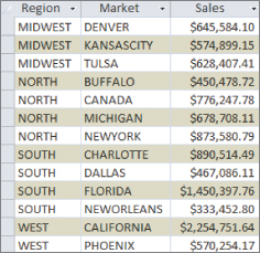
Figure 14.7 This dataset shows revenue by region and market.
A second SELECT statement produces a separate dataset (see Figure 14.8) that shows total revenue by region.
SELECT Region, "Total" AS [Market], Sum(Revenue) AS [Sales]
FROM PvTblFeed
GROUP BY Region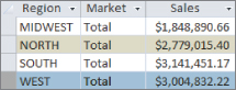
Figure 14.8 This dataset shows total revenue by region.
The idea is to bring together these two datasets to create an analysis that will show detail and totals all in one table. The UNION operator is ideal for this type of work, merging the results of the two SELECT statements. To use the UNION operator, simply start a new query, switch to SQL view, and enter the following syntax:
SELECT Region, Market, Sum(Revenue) AS [Sales]
FROM PvTblFeed
GROUP BY Region, Market
UNION
SELECT Region, "Total" AS [Market], Sum(Revenue) AS [Sales]
FROM PvTblFeed
GROUP BY Region
As you can see, the preceding statement is nothing more than the two SQL statements brought together with a UNION operator. When the two are merged (see Figure 14.9), the result is a dataset that shows both details and totals in one table!

Figure 14.9 The two datasets have now been combined to create a report that provides summary and detail data.
Creating a table with the CREATE TABLE statement
Often in your analytical processes, you'll need to create a temporary table in order to group, manipulate, or simply hold data. The CREATE TABLE statement allows you to do just that with one SQL-specific query.
Unlike a make-table query, the CREATE TABLE statement is designed to create only the structure or schema of a table. No records are ever returned with a CREATE TABLE statement. This statement allows you to strategically create an empty table at any point in your analytical process.
The basic syntax for a CREATE TABLE statement is as follows:
CREATE TABLE TableName
(<Field1Name> Type(<Field Size>), <Field2Name> Type(<Field Size>))
To use the CREATE TABLE statement, simply start a new query, switch to SQL view, and define the structure for your table.
In the following example, a new table called TempLog is created with three fields. The first field is a Text field that can accept 50 characters, the second field is a Text field that can accept 255 characters, and the third field is a Date field.
CREATE TABLE TempLog
([User] Text(50), [Description] Text, [LogDate] Date)Manipulating columns with the ALTER TABLE statement
The ALTER TABLE statement provides some additional methods of altering the structure of a table behind the scenes. There are several clauses you can use with the ALTER TABLE statement, four of which are quite useful in Access data analysis: ADD, ALTER COLUMN, DROP COLUMN, and ADD CONSTRAINT.
Adding a column with the ADD clause
As the name implies, the ADD clause enables you to add a column to an existing table. The basic syntax is as follows:
ALTER TABLE <TableName>
ADD <ColumnName> Type(<Field Size>)
To use the ADD statement, simply start a new query in SQL view and define the structure for your new column. For instance, running the example statement shown here will create a new column called SupervisorPhone that is being added to a table called TempLog:
ALTER TABLE TempLog
ADD SupervisorPhone Text(10)
Altering a column with the ALTER COLUMN clause
When using the ALTER COLUMN clause, you specify an existing column in an existing table. This clause is used primarily to change the data type and field size of a given column. The basic syntax is as follows:
ALTER TABLE <TableName>
ALTER COLUMN <ColumnName> Type(<Field Size>)
To use the ALTER COLUMN statement, simply start a new query in SQL view and define changes for the column in question. For instance, the example statement shown here will change the field size of the SupervisorPhone field:
ALTER TABLE TempLog
ALTER COLUMN SupervisorPhone Text(13)
Deleting a column with the DROP COLUMN clause
The DROP COLUMN clause enables you to delete a given column from an existing table. The basic syntax is as follows:
ALTER TABLE <TableName>
DROP COLUMN <ColumnName>
To use the DROP COLUMN statement, simply start a new query in SQL view and define the structure for your new column. For instance, running the example statement shown here will delete the column called SupervisorPhone from the TempLog table:
ALTER TABLE TempLog
DROP COLUMN SupervisorPhone
Dynamically adding primary keys with the ADD CONSTRAINT clause
For many analysts, Access serves as an easy to use extract, transform, load (ETL) tool. That is, Access allows you to extract data from many sources, and then reformat and cleanse that data into consolidated tables. Many analysts also automate ETL processes with the use of macros that fire a series of queries. This works quite well in most cases.
There are, however, instances in which an ETL process requires primary keys to be added to temporary tables in order to keep data normalized during processing. In these situations, most people do one of two things: They stop the macro in the middle of processing to manually add the required primary keys, or they create a permanent table solely for the purpose of holding a table where the primary keys are already set.
There is a third option, though: The ADD CONSTRAINT clause allows you to dynamically create the primary keys. The basic syntax is as follows:
ALTER TABLE <TableName>
ADD CONSTRAINT ConstraintName PRIMARY KEY (<Field Name>)
To use the ADD CONSTRAINT clause, simply start a new query in SQL view and define the new primary key you're implementing. For instance, the example statement shown here will apply a compound key to three fields in the TempLog table.
ALTER TABLE TempLog
ADD CONSTRAINT ConstraintName PRIMARY KEY (ID, Name, Email)
Creating pass-through queries
A pass-through query sends SQL commands directly to a database server (such as SQL Server, Oracle, and so on). Often these database servers are known as the back end of the system, with Access being the client tool or front end. You send the command by using the syntax required by the particular server.
The advantage of pass-through queries is that the parsing and processing is actually done on the back-end server, not in Access. This makes them much faster than queries that pull from linked tables, particularly if the linked table is a very large one.
Here are the steps for building a pass-through query:
- On the Create tab of the Ribbon, click the Query Design command.
- Close the Show Table dialog box.
- Click the Pass-Through command on the Query Tools Design tab. The SQL design window appears.
- Type a SQL statement that is appropriate for the target database system. Figure 14.10 demonstrates a simple SQL statement.
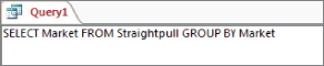
Figure 14.10 To create a pass-through query, you must use the SQL window.
- On the Query Tools Design tab, click the Property Sheet command. The Property Sheet dialog box (shown in Figure 14.11) appears.
![Screenshot of Property Sheet dialog box presenting the General tab with ODBC Connection String input ODBC;Driver=[SQL Server]; Server=,mssql501.ixwebhosting.com;Database=mkt0a0h_traning.](http://images-20200215.ebookreading.net/22/4/4/9781119086543/9781119086543__access-2016-bible__9781119086543__images__c14f011.jpg)
Figure 14.11 You must specify an ODBC connection string in the pass-through query's Property Sheet dialog box.
- Enter the appropriate connection string for your server. This is typically the ODBC connection string you normally use to connect to your server.
- Click Run.
There are a few things you should be aware of when choosing to go the pass-through query route:
- You'll have to build the SQL statements yourself. Access provides no help—you can't use the QBE to build your statement.
- If the connection string of your server changes, you'll have to go back into the properties of the pass-through query and edit the ODBC connection string property. Alternatively, if you are using an existing DSN, you can simply edit the DSN configuration.
- The results you get from a pass-through are read only. You can't update or edit the returned records.
- You can only write queries that select data. This means you can't write update, append, delete, or make-table queries.
- Because you're hard-coding the SQL statements that will be sent to the server, including dynamic parameters (like a parameter query) is impossible because there is no way to get your parameters to the server after the SQL statement is sent.