
Chapter 12
Working with Calculations and Dates
IN THIS CHAPTER
- Using calculations in your analyses
- Using dates in your analyses
The truth is that few organizations can analyze their raw data at face value. More often than not, some preliminary analysis with calculations and dates must be carried out before the big-picture analysis can be performed. As you'll learn in this chapter, Access provides a wide array of tools and built-in functions that make working with calculations and dates possible.
Using Calculations in Your Analyses
If you're an Excel user trying to familiarize yourself with Access, one of the questions you undoubtedly have is, “Where do the formulas go?” In Excel, you have the flexibility to enter a calculation via a formula directly into the dataset you're analyzing. You can't do this in Access. So, the question is, “Where do you store calculations in Access?”
As you've already learned, things work differently in Access. A best practice when working in a database environment is to keep your data separate from your analysis. In this light, you won't be able to store a calculation (a formula) in your dataset. Now, it's true that you can store the calculated results in your tables, but using tables to store calculated results is problematic for several reasons:
- Stored calculations take up valuable storage space.
- Stored calculations require constant maintenance as the data in your table changes.
- Stored calculations generally tie your data to one analytical path.
Instead of storing the calculated results as hard data, it's a better practice to perform calculations in real time, at the precise moment when they're needed. This ensures the most current and accurate results and doesn't tie your data to one particular analysis.
Common calculation scenarios
In Access, calculations are performed using expressions. An expression is a combination of values, operators, or functions that are evaluated to return a separate value to be used in a subsequent process. For example, 2+2 is an expression that returns the integer 4, which can be used in a subsequent analysis. Expressions can be used almost anywhere in Access to accomplish various tasks: in queries, forms, reports, data access pages, and even tables to a certain degree. In this section, you'll learn how to expand your analysis by building real-time calculations using expressions.
Using constants in calculations
Most calculations typically consist of hard-coded numbers or constants. A constant is a static value that doesn't change. For example, in the expression [List_Price]*1.1, 1.1 is a constant; the value of 1.1 will never change. Figure 12.1 demonstrates how a constant can be used in an expression within a query.
![Screenshot of query design window displaying OrderDate, WarningDate: DateAdd(“ww”,3,[OrderDate]), and Overdue Date: DateAdd(“m”,1,[OrderDate])are entered in Field cells (left-right). of a query design set to group the records by product name and calculate the sum of workday sales for each market. <>7 And <>1, 2013, and Is Null are the criteria for weekday, year, and holidays. of query design window displaying ForecastSummary table. Market and DollarVariance: [Actual]-[Forecast] are entered in Field cells in columns 1 and 2, respectively.](http://images-20200215.ebookreading.net/22/4/4/9781119086543/9781119086543__access-2016-bible__9781119086543__images__c12f001.jpg)
Figure 12.1 In this query, you're using a constant to calculate a 10 percent price increase.
In this example, you're building a query that will analyze how the current price for each product compares to the same price with a 10 percent increase. The expression, entered under the alias “Increase” will multiply the List_Price field of each record with a constant value of 1.1, calculating a price that is 10 percent over the original value in the List_Price field.
Using fields in calculations
Not all your calculations will require you to specify a constant. In fact, many of the mathematical operations you'll carry out will be performed on data that already resides in fields within your dataset. You can perform calculations using any fields formatted as number or currency.
For instance, in the query shown in Figure 12.2, you aren't using any constants. Instead, your calculation will be executed using the values in each record of the dataset. This is similar to referencing cell values in an Excel formula.
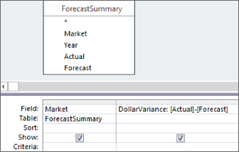
Figure 12.2 In this query, you're using two fields in a Dollar Variance calculation.
Using the results of aggregation in calculations
Using the result of an aggregation as an expression in a calculation allows you to perform multiple analytical steps in one query. In the example in Figure 12.3, you're running an aggregate query. This query will execute in the following order:
![Screenshot of query design window displaying ForecastSummary table. Market, AdjustedForecast: [Forecast]*0.9, and NewVariance: [Actual]-[AdjustedForecast] are added in the Field cells (left-right).](http://images-20200215.ebookreading.net/22/4/4/9781119086543/9781119086543__access-2016-bible__9781119086543__images__c12f003.jpg)
Figure 12.3 In this query, you're using the aggregation results for each market as expressions in your calculation.
- The query groups your records by market.
- The query calculates the count of orders and the sum of revenue for each market.
- The query assigns the aliases you've defined respectively (OrderCount and Rev).
- The query uses the aggregation results for each branch as expressions in your AvgDollarPerOrder calculation.
Using the results of one calculation as an expression in another
Keep in mind that you aren't limited to one calculation per query. In fact, you can use the results of one calculation as an expression in another calculation. Figure 12.4 illustrates this concept.
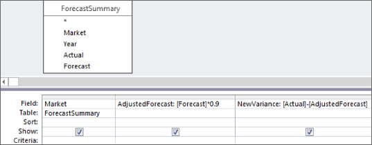
Figure 12.4 This query uses the results of one calculation as an expression in another.
In this query, you're first calculating an adjusted forecast, and then you're using the results of that calculation in another calculation that returns the variance of actual versus adjusted forecast.
Using a calculation as an argument in a function
Look at the query in Figure 12.5. The calculation in this query will return a number with a fractional part. That is, it will return a number that contains a decimal point followed by many trailing digits. You would like to return a round number, however, making the resulting dataset easier to read.
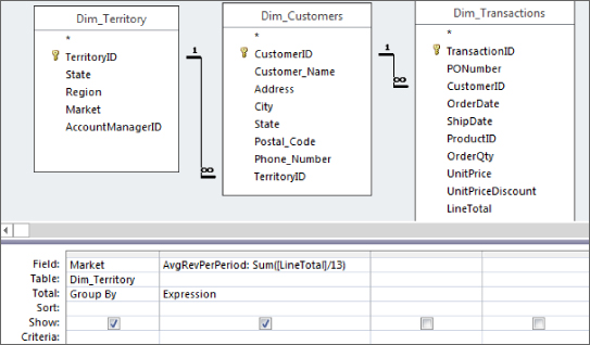
Figure 12.5 The results of this calculation will be difficult to read because they'll all be fractional numbers that have many digits trailing a decimal point. Forcing the results into round numbers will make for easier reading.
To force the results of your calculation into an integer, you can use the Int function. The Int function is a mathematical function that will remove the fractional part of a number and return the resulting integer. This function takes one argument, a number. However, instead of hard-coding a number into this function, you can use your calculation as the argument. Figure 12.6 demonstrates this concept.

Figure 12.6 You can use your calculation as the argument in the Int function, allowing you to remove the fractional part from the resulting data.
Constructing calculations with the Expression Builder
If you aren't yet comfortable manually creating complex expressions with functions and calculations, Access provides the Expression Builder. The Expression Builder guides you through constructing an expression with a few clicks of the mouse. Avid Excel users may relate the Expression Builder to the Insert Function Wizard found in Excel. The idea is that you build your expression simply by selecting the necessary functions and data fields.
To activate the Expression Builder, click inside the query grid cell that will contain your expression, right-click, and then select Build, as shown in Figure 12.7.

Figure 12.7 Activate the Expression Builder by right-clicking inside the Field row of the query grid and selecting Build.
As you can see in Figure 12.8, the Expression Builder has four panes to work in. The upper pane is where you enter the expression. The lower panes show the different objects available to you. In the lower-left pane you can use the plus icons to expose the database objects that can be used to build out your expression.

Figure 12.8 The Expression Builder will display any database object you can use in your expression.
Double-click any of the database objects to drill down to the next level of objects. By double-clicking the Functions object, for example, you'll be able to drill into the Built-In Functions folder where you'll see all the functions available to you in Access. Figure 12.9 shows the Expression Builder set to display all the available math functions.

Figure 12.9 The Expression Builder displays all the functions available to you.
The idea is that you double-click the function you need and Access will automatically enter the function in the upper pane of the Expression Builder. In the example shown in Figure 12.10, the selected function is the Round function. As you can see, the function is immediately placed in the upper pane of the Expression Builder, and Access shows you the arguments needed to make the function work. In this case, there are two arguments identified: a Number argument and a Precision argument.
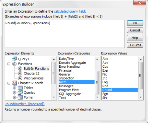
Figure 12.10 Access tells you which arguments are needed to make the function work.
If you don't know what an argument means, simply highlight the argument in the upper pane and then click the hyperlink at the bottom of the dialog box (see Figure 12.11). A Help window provides an explanation of the function.
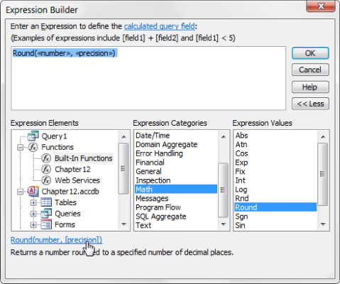
Figure 12.11 Help files are available to explain each function in detail.
As you can see in Figure 12.12, instead of using a hard-coded number in the Round function, an expression is used to return a dynamic value. This calculation will divide the sum of [Dim_Transactions]![LineTotal] by 13. Since the Precision argument is optional, that argument is left off.
![Screenshot of query design window displaying Dim_Transactions table. Expr1: Round([Dim_Transactions]![LineTotal]/13) is entered in the Field cell and Sum is entered in the Total cell.](http://images-20200215.ebookreading.net/22/4/4/9781119086543/9781119086543__access-2016-bible__9781119086543__images__c12f012.jpg)
Figure 12.12 The function here will round the results of the calculation, ([Dim_Transactions]![Line Total])/13.
When you're satisfied with your newly created expression, click OK to insert it into the query grid. Figure 12.13 shows that the new expression has been added as a field. Note that the new field has a default alias of Expr1; you can rename this to something more meaningful.
![Screenshot of query design window displaying ForecastSummary table. Market, Actual, Forecast, and Variance: [Actual]-[Forecast] are entered in Field cells (left to right).](http://images-20200215.ebookreading.net/22/4/4/9781119086543/9781119086543__access-2016-bible__9781119086543__images__c12f013.jpg)
Figure 12.13 Your newly created expression will give you the average revenue per period for all transactions.
Common calculation errors
No matter which platform you're using to analyze your data, there's always the risk of errors when working with calculations. There is no magic function in Access that will help you prevent errors in your analysis. However, there are a few fundamental actions you can take to avoid some of the most common calculation errors.
Understanding the order of operator precedence
You might remember from your algebra days that when working with a complex equation, executing multiple mathematical operations, the equation does not necessarily evaluate from left to right. Some operations have precedence over others and therefore must occur first. The Access environment has similar rules regarding the order of operator precedence. When you're using expressions and calculations that involve several operations, each operation is evaluated and resolved in a predetermined order. It's important to know the order of operator precedence in Access. An expression that is incorrectly built may cause errors on your analysis.
The order of operations for Access is as follows:
- Evaluate items in parentheses.
- Perform exponentiation (
^calculates exponents). - Perform negation (
-converts to negative). - Perform multiplication (
*multiplies) and division (/divides) at equal precedence. - Perform addition (
+adds) and subtraction (-subtracts) at equal precedence. - Evaluate string concatenation (
&). - Evaluate comparison and pattern matching operators (
>,<,=,<>,>=,<=,Like,Between,Is) at equal precedence. - Evaluate logical operators in the following order:
Not,And,Or.
How can understanding the order of operations ensure that you avoid analytical errors? Consider this basic example: The correct answer to the calculation, (20+30)*4, is 200. However, if you leave off the parentheses—as in 20+30*4—Access will perform the calculation like this: 30*4 = 120 + 20 = 140. The order of operator precedence mandates that Access perform multiplication before subtraction. Therefore, entering 20+30*4 will give you the wrong answer. Because the order of operator precedence in Access mandates that all operations in parentheses be evaluated first, placing 20+30 inside parentheses ensures the correct answer.
Watching out for null values
A null value represents the absence of any value. When you see a data item in an Access table that is empty or has no information in it, it is considered null.
If Access encounters a null value, it doesn't assume that the null value represents zero; instead, it immediately returns a null value as the answer. To illustrate this behavior, build the query shown in Figure 12.14.
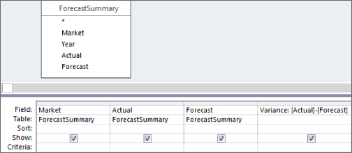
Figure 12.14 To demonstrate how null values can cause calculation errors, build this query in Design view.
Run the query, and you'll see the results shown in Figure 12.15. Notice that the Variance calculation for the first record doesn't show the expected results; instead, it shows a null value. This is because the forecast value for that record is a null value.
![Screenshot of query design window displaying ForecastSummary table. Market, Actual, Forecast, and Variance: [Actual]-Nz([Forecast],0) are entered in Field cells (left to right).](http://images-20200215.ebookreading.net/22/4/4/9781119086543/9781119086543__access-2016-bible__9781119086543__images__c12f015.jpg)
Figure 12.15 When any variable in your calculation is null, the resulting answer is a null value.
Looking at Figure 12.15, you can imagine how a null calculation error can wreak havoc on your analysis, especially if you have an involved analytical process. Furthermore, null calculation errors can be difficult to identify and fix.
That being said, you can avoid null calculation errors by using the Nz function, which enables you to convert any null value that is encountered to a value you specify:
Nz(variant, valueifnull)The Nz function takes two arguments:
variant: The data you're working withvalueifnull: The value you want returned if the variant is null
Nz([MyNumberField],0) converts any null value in MyNumberField to zero.
Because the problem field is the Forecast field, you would pass the Forecast field through the Nz function. Figure 12.16 shows the adjusted query.
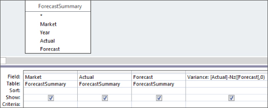
Figure 12.16 Pass the Forecast field through the Nz function to convert null values to zero.
As you can see in Figure 12.17, the first record now shows a variance value even though the values in the Forecast field are null. Note that the Nz function did not physically place a zero in the null values. The Nz function merely told access to treat the nulls as zeros when calculating the Variance field.
![Screenshot of query design window displaying Dim_Transactions table. ShipDate and NewShipDate: [ShipDate]+30 are entered in Field cells (left to right).](http://images-20200215.ebookreading.net/22/4/4/9781119086543/9781119086543__access-2016-bible__9781119086543__images__c12f017.jpg)
Figure 12.17 The first record now shows a variance value.
Watching the syntax in your expressions
Basic syntax mistakes in your calculation expressions can also lead to errors. Follow these basic guidelines to avoid slip-ups:
- If you're using fields in your calculations, enclose their names in square brackets (
[]). - Make sure you spell the names of the fields correctly.
- When assigning an alias to your calculated field, be sure you don't inadvertently use a field name from any of the tables being queried.
- Don't use illegal characters—period (
.), exclamation point (!), square brackets ([]) or ampersand (&)—in your aliases.
Using Dates in Your Analyses
In Access, every possible date starting from December 31, 1899, is stored as a positive serial number. For example, December 31, 1899, is stored as 1; January 1, 1900, is stored as 2; and so on. This system of storing dates as serial numbers, commonly called the 1900 system, is the default date system for all Office applications. You can take advantage of this system to perform calculations with dates.
Simple date calculations
Figure 12.18 shows one of the simplest calculations you can perform on a date. In this query, you're adding 30 to each ship date. This will effectively return the order date plus 30 days, giving you a new date.
![Screenshot of query design window displaying Dim_Transactions table. DaysToShip: [ShipDate]-[OrderDate] is entered in the Field cell.](http://images-20200215.ebookreading.net/22/4/4/9781119086543/9781119086543__access-2016-bible__9781119086543__images__c12f018.jpg)
Figure 12.18 You're adding 30 to each ship date, effectively creating a date that is equal to the ship date plus 30 days.
You can also calculate the number of days between two dates. The calculation in Figure 12.19, for example, essentially subtracts the serial number of one date from the serial number of another date, leaving you the number of days between the two dates.
![Screenshot of query design window displaying Dim_Transactions table. PONumber and DaysOld: Date0-[OrderDate] is entered in the Field cell.](http://images-20200215.ebookreading.net/22/4/4/9781119086543/9781119086543__access-2016-bible__9781119086543__images__c12f019.jpg)
Figure 12.19 In this query, you're calculating the number of days between two dates.
Advanced analysis using functions
There are 25 built-in date/time functions available in Access 2016. Some of these are functions you'll very rarely encounter, whereas others you'll use routinely in your analyses. This section discusses a few of the basic date/time functions that will come in handy in your day-to-day analysis.
The Date function
The Date function is a built-in Access function that returns the current system date—in other words, today's date. With this versatile function, you never have to hard-code today's date in your calculations. That is, you can create dynamic calculations that use the current system date as a variable, giving you a different result every day. In this section, we look at some of the ways you can leverage the Date function to enhance your analysis.
Finding the number of days between today and a past date
Imagine that you have to calculate aged receivables. You need to know the current date to determine how overdue the receivables are. Of course, you could type in the current date by hand, but that can be cumbersome and prone to error.
To demonstrate how to use the Date function, create the query shown in Figure 12.20.

Figure 12.20 This query returns the number of days between today's date and each order date.
Using the Date function in a criteria expression
You can use the Date function to filter out records by including it in a criteria expression. For example, the query shown in Figure 12.21 will return all records with an order date older than 90 days.
![Screenshot of query design window displaying Dim_AccountManagers table. FullName and YearsEmployed: Date0-[HireDate] are entered in Field cells (left-right).](http://images-20200215.ebookreading.net/22/4/4/9781119086543/9781119086543__access-2016-bible__9781119086543__images__c12f021.jpg)
Figure 12.21 No matter what day it is today, this query will return all orders older than 90 days.
Calculating an age in years using the Date function
Imagine that you've been asked to provide a list of account managers along with the number of years they have been employed by the company. To accomplish this task, you have to calculate the difference between today's date and each manager's hire date.
The first step is to build the query shown in Figure 12.22.

Figure 12.22 You're calculating the difference between today's date and each manager's hire date.
When you look at the query results, shown in Figure 12.23, you'll realize that the calculation results in the number of days between the two dates, not the number of years.
![Screenshot of query design window displaying Dim_AccountManagers table. FullName and YearsEmployed: (Date0-[HireDate])/365.25 are entered in Field cells (left-right).](http://images-20200215.ebookreading.net/22/4/4/9781119086543/9781119086543__access-2016-bible__9781119086543__images__c12f023.jpg)
Figure 12.23 This dataset shows the number of days, not the number of years.
To fix this problem, switch back to Design view and divide your calculation by 365.25. Why 365.25? That's the average number of days in a year when you account for leap years. Figure 12.24 demonstrates this change. Note that your original calculation is now wrapped in parentheses to avoid errors due to order of operator precedence.

Figure 12.24 Divide your original calculation by 365.25 to convert the answer to years.
A look at the results, shown in Figure 12.25, proves that you're now returning the number of years. All that's left to do is to strip away the fractional portion of the date using the Int function. Why the Int function? The Int function doesn't round the year up or down; it merely converts the number to a readable integer.
![Screenshot of query design window displaying Dim_AccountManagers table. FullName and YearsEmployed: Int((Date0-[HireDate])/365.25) are entered in Field cells (left-right).](http://images-20200215.ebookreading.net/22/4/4/9781119086543/9781119086543__access-2016-bible__9781119086543__images__c12f025.jpg)
Figure 12.25 Your query is now returning years, but you have to strip away the fractional portion of your answer.
Wrapping your calculation in the Int function ensures that your answer will be a clean year without fractions (see Figure 12.26).
![Screenshot of query design window displaying Year: Year([OrderDate]), Month: Month([OrderDate]), Day: Day([OrderDate]), and Weekday: Weekday([OrderDate]) entered in Field cells (left-right).](http://images-20200215.ebookreading.net/22/4/4/9781119086543/9781119086543__access-2016-bible__9781119086543__images__c12f026.jpg)
Figure 12.26 Running this query will return the number of years each employee has been with the company.
The Year, Month, Day, and Weekday functions
The Year, Month, Day, and Weekday functions are used to return an integer that represents their respective parts of a date. All these functions require a valid date as an argument. For example:
Year(#12/31/2013#)returns2013.Month(#12/31/2013#)returns12.Day(#12/31/2013#)returns31.Weekday(#12/31/2013#)returns3.
Figure 12.27 demonstrates how you would use these functions in a query environment.

Figure 12.27 The Year, Month, Day, and Weekday functions enable you to parse out a part of a date.
The DateAdd function
A common analysis for many organizations is to determine on which date a certain benchmark will be reached. For example, most businesses want to know on what date an order will become 30 days past due. Furthermore, what date should a warning letter be sent to the customer? An easy way to perform these types of analyses is to use the DateAdd function, which returns a date to which a specified interval has been added:
DateAdd(interval, number, date)The DateAdd function returns a date to which a specified interval has been added. There are three required arguments in the DateAdd function.
interval(required): The interval of time you want to use. The intervals available are as follows:"yyyy": Year"q": Quarter"m": Month"y": Day of year"d": Day"w": Weekday"ww": Week"h": Hour"n": Minute"s": Second
number(required): The number of intervals to add. A positive number returns a date in the future, whereas a negative number returns a date in the past.date(required): The date value with which you're working. For example:DateAdd("ww",1,#11/30/2013#)returns 12/7/2013.DateAdd("m",2,#11/30/2013#)returns 1/30/2014.DateAdd("yyyy",-1,#11/30/2013#)returns 11/30/2012.
The query shown in Figure 12.28 illustrates how the DateAdd function can be used in determining the exact date a specific benchmark is reached. You're creating two new fields with this query: Warning and Overdue. The DateAdd function used in the Warning field will return the date that is three weeks from the original order date. The DateAdd function used in the Overdue field will return the date that is one month from the original order date.
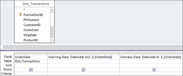
Figure 12.28 This query will give you the original order date, the date you should send a warning letter, and the date on which the order will be 30 days overdue.
Grouping dates into quarters
Why would you need to group your dates into quarters? Most databases store dates rather than quarter designations. Therefore, if you wanted to analyze data on a quarter-over-quarter basis, you would have to convert dates into quarters. Surprisingly, there is no date/time function that allows you to group dates into quarters. There is, however, the Format function.
The Format function belongs to the Text category of functions and allows you to convert a variant into a string based on formatting instructions. From the perspective of analyzing dates, there are several valid instructions you can pass to a Format function:
Format(#01/31/2013#, "yyyy")returns2013.Format(#01/31/2013#, "yy")returns13.Format(#01/31/2013#, "q")returns1.Format(#01/31/2013#, "mmm")returnsJan.Format(#01/31/2013#, "mm")returns01.Format(#01/31/2013#, "d")returns31.Format(#01/31/2013#, "w")returns5.Format(#01/31/2013#, "ww")returns5.
The query in Figure 12.29 shows how you would group all the order dates into quarters and then group the quarters to get a sum of revenue for each quarter.
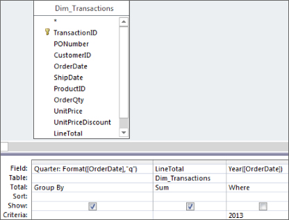
Figure 12.29 You can group dates into quarters by using the Format function.
If you want to get fancy, you can insert the Format function in a crosstab query, using Quarter as the column (see Figure 12.30).
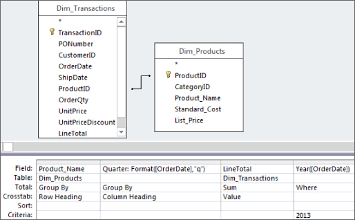
Figure 12.30 You can also use the Format function in a crosstab query.
As you can see in Figure 12.31, the resulting dataset is a clean look at revenue by product by quarter.

Figure 12.31 You've successfully grouped your dates into quarters.
The DateSerial function
The DateSerial function allows you to construct a date value by combining given year, month, and day components. This function is perfect for converting disparate strings that, together, represent a date, into an actual date.
DateSerial(Year, Month, Day)The DateSerial function has three arguments:
- Year (required): Any number or numeric expression from 100 to 9999
- Month (required): Any number or numeric expression
- Day (required): Any number or numeric expression
For example, the following statement would return April 3, 2012.
DateSerial(2012, 4, 3)So, how is this helpful? Well, now you can put a few twists on this by performing calculations on the expressions within the DateSerial function. Consider some of the possibilities:
- Get the first day of last month by subtracting
1from the current month and using1as theDayargument:DateSerial(Year(Date()), Month(Date()) - 1, 1) - Get the first day of next month by adding
1to the current month and using1as theDayargument:DateSerial(Year(Date()), Month(Date()) + 1, 1) - Get the last day of this month by adding
1to the current month and using0as theDayargument:DateSerial(Year(Date()), Month(Date())+1, 0) - Get the last day of next month by adding
2to the current month and using0as theDayargument:DateSerial(Year(Date()), Month(Date()) +2, 0)