
Chapter 6
Multivariate Statistics
So far we have discussed inference methods for one variable at a time. Data analysts are also interested in multivariate inferential methods, where the relationships between two variables, or between one target variable and a set of predictor variables, are analyzed.
We begin with bivariate analysis, where we have two independent samples and wish to test for significant differences in the means or proportions of the two samples. When would data miners be interested in using bivariate analysis? In Chapter 6, we illustrate how the data is partitioned into a training data set and a test data set for cross-validation purposes. Data miners can use the hypothesis tests shown here to determine whether significant differences exist between the means of various variables in the training and test data sets. If such differences exist, then the cross-validation is invalid, because the training data set is nonrepresentative of the test data set.
- For a continuous variable, use the two-sample t-test for the difference in means.
- For a flag variable, use the two-sample Z-test for the difference in proportions.
- For a multinomial variable, use the test for the homogeneity of proportions.
Of course, there are presumably many variables in each of the training set and test set. However, spot-checking of a few randomly chosen variables is usually sufficient.
6.1 Two-Sample t-Test for Difference in Means
To test for the difference in population means, we use the following test statistic:

which follows an approximate t distribution with degrees of freedom the smaller of ![]() and
and ![]() , whenever either both populations are normally distributed or both samples are large.
, whenever either both populations are normally distributed or both samples are large.
For example, we partitioned the churn data set into a training set of 2529 records and a test set of 804 records (the reader's partition will differ). We would like to assess the validity of the partition by testing whether the population mean number of customer service calls differs between the two data sets. The summary statistics are given in Table 6.1.
Table 6.1 Summary statistics for customer service calls, training data set, and test data set
| Data Set | Sample Mean | Sample Standard Deviation | Sample Size |
| Training set | |||
| Test set |
Now, the sample means do not look very different, but we would like to have the results of the hypothesis test just to make sure. The hypotheses are
The test statistic is

The two-tailed p-value for ![]() is
is
Since the p-value is large, there is no evidence that the mean number of customer service calls differs between the training data set and the test data set. For this variable at least, the partition seems valid.
6.2 Two-Sample Z-Test for Difference in Proportions
Of course not all variables are numeric, like customer service calls. What if we have a 0/1 flag variable – such as membership in the Voice Mail Plan – and wish to test whether the proportions of records with value 1 differ between the training data set and test data set? We could turn to the two-sample Z-test for the difference in proportions. The test statistic is
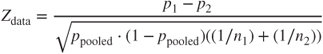
where ![]() , and
, and ![]() and
and ![]() represents the number of and proportion of records with value 1 for sample i, respectively.
represents the number of and proportion of records with value 1 for sample i, respectively.
For example, our partition resulted in ![]() of
of ![]() customers in the training set belonging to the Voice Mail Plan, while
customers in the training set belonging to the Voice Mail Plan, while ![]() of
of ![]() customers in the test set belonging, so that
customers in the test set belonging, so that ![]() ,
, ![]() , and
, and ![]() .
.
The hypotheses are
The test statistic is

The p-value is
Thus, there is no evidence that the proportion of Voice Mail Plan members differs between the training and test data sets. For this variable, the partition is valid.
6.3 Test for the Homogeneity of Proportions
Multinomial data is an extension of binomial data to k > 2 categories. For example, suppose a multinomial variable marital status takes the values married, single, and other. Suppose we have a training set of 1000 people and a test set of 250 people, with the frequencies shown in Table 6.2.
Table 6.2 Observed frequencies
| Data Set | Married | Single | Other | Total |
| Training set | 410 | 340 | 250 | 1000 |
| Test set | 95 | 85 | 70 | 250 |
| Total | 505 | 425 | 320 | 1250 |
To determine whether significant differences exist between the multinomial proportions of the two data sets, we could turn to the test for the homogeneity of proportions.1 The hypotheses are

To determine whether these observed frequencies represent proportions that are significantly different for the training and test data sets, we compare these observed frequencies with the expected frequencies that we would expect if ![]() were true. For example, to find the expected frequency for the number of married people in the training set, we (i) find the overall proportion of married people in both the training and test sets,
were true. For example, to find the expected frequency for the number of married people in the training set, we (i) find the overall proportion of married people in both the training and test sets, ![]() , and (ii) we multiply this overall proportion by the number of people in the training set, 1000, giving us the expected proportion of married people in the training set to be
, and (ii) we multiply this overall proportion by the number of people in the training set, 1000, giving us the expected proportion of married people in the training set to be
We use the overall proportion in (i) because ![]() states that the training and test proportions are equal. Generalizing, for each cell in the table, the expected frequencies are calculated as follows:
states that the training and test proportions are equal. Generalizing, for each cell in the table, the expected frequencies are calculated as follows:
Applying this formula to each cell in the table gives us the table of expected frequencies in Table 6.3.
Table 6.3 Expected frequencies
| Data Set | Married | Single | Other | Total |
| Training set | 404 | 340 | 256 | 1000 |
| Test set | 101 | 85 | 64 | 250 |
| Total | 505 | 425 | 320 | 1250 |
The observed frequencies (O) and the expected frequencies (E) are compared using a test statistic from the ![]() (chi-square) distribution:
(chi-square) distribution:
Large differences between the observed and expected frequencies, and thus a large value for ![]() , will lead to a small p-value, and a rejection of the null hypothesis. Table 6.4 illustrates how the test statistic is calculated.
, will lead to a small p-value, and a rejection of the null hypothesis. Table 6.4 illustrates how the test statistic is calculated.
Table 6.4 Calculating the test statistic ![]()
| Cell | Observed Frequency | Expected Frequency | |
| Married, training | 410 | 404 | |
| Married, test | 95 | 101 | |
| Single, training | 340 | 340 | |
| Single, test | 85 | 85 | |
| Other, training | 250 | 256 | |
| Other, test | 70 | 64 | |
The p-value is the area to the right of ![]() under the
under the ![]() curve with degrees of freedom equal to (number of rows − 1) (number of columns − 1) = (1)(2) = 2:
curve with degrees of freedom equal to (number of rows − 1) (number of columns − 1) = (1)(2) = 2:
Because this p-value is large, there is no evidence that the observed frequencies represent proportions that are significantly different for the training and test data sets. In other words, for this variable, the partition is valid.
This concludes our coverage of the tests to apply when checking the validity of a partition.
6.4 Chi-Square Test for Goodness of Fit of Multinomial Data
Next, suppose a multinomial variable marital status takes the values married, single, and other, and suppose that we know that 40% of the individuals in the population are married, 35% are single, and 25% report another marital status. We are taking a sample and would like to determine whether the sample is representative of the population. We could turn to the ![]() (chi-square) goodness of fit test.
(chi-square) goodness of fit test.
The hypotheses for this ![]() goodness of fit test would be as follows:
goodness of fit test would be as follows:

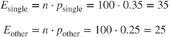
Our sample of size n = 100, yields the following observed frequencies (represented by the letter “O”):
To determine whether these counts represent proportions that are significantly different from those expressed in ![]() , we compare these observed frequencies with the expected frequencies that we would expect if
, we compare these observed frequencies with the expected frequencies that we would expect if ![]() were true. If
were true. If ![]() were true, then we would expect 40% of our sample of 100 individuals to be married, that is, the expected frequency for married is
were true, then we would expect 40% of our sample of 100 individuals to be married, that is, the expected frequency for married is
Similarly,
These frequencies are compared using the test statistic:
Again, large differences between the observed and expected frequencies, and thus a large value for ![]() , will lead to a small p-value, and a rejection of the null hypothesis. Table 6.5 illustrates how the test statistic is calculated.
, will lead to a small p-value, and a rejection of the null hypothesis. Table 6.5 illustrates how the test statistic is calculated.
Table 6.5 Calculating the test statistic ![]()
| Marital Status | Observed Frequency | Expected Frequency | |
| Married | 36 | 40 | |
| Single | 35 | 35 | |
| Other | 29 | 25 | |
The p-value is the area to the right of ![]() under the
under the ![]() curve with k − 1 degrees of freedom, where k is the number of categories (here k = 3):
curve with k − 1 degrees of freedom, where k is the number of categories (here k = 3):
Thus, there is no evidence that the observed frequencies represent proportions that differ significantly from those in the null hypothesis. In other words, our sample is representative of the population.
6.5 Analysis of Variance
In an extension of the situation for the two-sample t-test, suppose that we have a threefold partition of the data set, and wish to test whether the mean value of a continuous variable is the same across all three subsets. We could turn to one-way analysis of variance (ANOVA). To understand how ANOVA works, consider the following small example. We have samples from Groups A, B, and C, of four observations each, for the continuous variable age, shown in Table 6.6.
Table 6.6 Sample ages for Groups A, B, and C
| Group A | Group B | Group C |
| 30 | 25 | 25 |
| 40 | 30 | 30 |
| 50 | 50 | 40 |
| 60 | 55 | 45 |
The hypotheses are

The sample mean ages are ![]() ,
, ![]() , and
, and ![]() . A comparison dot plot of the data (Figure 6.1) shows that there is a considerable amount of overlap among the three data sets. So, despite the difference in sample means, the dotplot offers little or no evidence to reject the null hypothesis that the population means are all equal.
. A comparison dot plot of the data (Figure 6.1) shows that there is a considerable amount of overlap among the three data sets. So, despite the difference in sample means, the dotplot offers little or no evidence to reject the null hypothesis that the population means are all equal.

Figure 6.1 Dotplot of Groups A, B, and C shows considerable overlap.
Next, consider the following samples from Groups D, E, and F, for the continuous variable age, shown in Table 6.7.
Table 6.7 Sample ages for Groups D, E, and F
| Group D | Group E | Group F |
| 43 | 37 | 34 |
| 45 | 40 | 35 |
| 45 | 40 | 35 |
| 47 | 43 | 36 |
Once again, the sample mean ages are ![]() ,
, ![]() , and
, and ![]() . A comparison dot plot of this data (Figure 6.2) illustrates that there is very little overlap among the three data sets. Thus, Figure 6.2 offers good evidence to reject the null hypothesis that the population means are all equal.
. A comparison dot plot of this data (Figure 6.2) illustrates that there is very little overlap among the three data sets. Thus, Figure 6.2 offers good evidence to reject the null hypothesis that the population means are all equal.

Figure 6.2 Dotplot of Groups D, E, and F shows little overlap.
To recapitulate, Figure 6.1 shows no evidence of difference in group means, while Figure 6.2 shows good evidence of differences in group means, even though the respective sample means are the same in both cases. The distinction stems from the overlap among the groups, which itself is a result of the spread within each group. Note that the spread is large for each group in Figure 6.1, and small for each group in Figure 6.2. When the spread within each sample is large (Figure 6.1), the difference in sample means seems small. When the spread within each sample is small (Figure 6.2), the difference in sample means seems large.
ANOVA works by performing the following comparison. Compare
- the between-sample variability, that is, the variability in the sample means, such as
 ,
,  , and
, and  , with
 - the within-sample variability, that is, the variability within each sample, measured, for example, by the sample standard deviations.
When (1) is much larger than (2), this represents evidence that the population means are not equal. Thus, the analysis depends on measuring variability, hence the term analysis of variance.
Let ![]() represent the overall sample mean, that is, the mean of all observations from all groups. We measure the between-sample variability by finding the variance of the k sample means, weighted by sample size, and expressed as the mean square treatment (MSTR):
represent the overall sample mean, that is, the mean of all observations from all groups. We measure the between-sample variability by finding the variance of the k sample means, weighted by sample size, and expressed as the mean square treatment (MSTR):
We measure the within-sample variability by finding the weighted mean of the sample variances, expressed as the mean square error (MSE):
We compare these two quantities by taking their ratio:
which follows an F distribution, with degrees of freedom ![]() and
and ![]() . The numerator of MSTR is the sum of squares treatment, SSTR, and the numerator of MSE is the sum of squares error, SSE. The total sum of squares (SST) is the sum of SSTR and SSE. A convenient way to display the above quantities is in the ANOVA table, shown in Table 6.8.
. The numerator of MSTR is the sum of squares treatment, SSTR, and the numerator of MSE is the sum of squares error, SSE. The total sum of squares (SST) is the sum of SSTR and SSE. A convenient way to display the above quantities is in the ANOVA table, shown in Table 6.8.
Table 6.8 ANOVA table
| Source of | Sum of | Degrees of | Mean | |
| Variation | Squares | Freedom | Square | F |
| Treatment | SSTR | |||
| Error | SSE | |||
| Total | SST |
The test statistic ![]() will be large when the between-sample variability is much greater than the within-sample variability, which is indicative of a situation calling for rejection of the null hypothesis. The p-value is
will be large when the between-sample variability is much greater than the within-sample variability, which is indicative of a situation calling for rejection of the null hypothesis. The p-value is ![]() ; reject the null hypothesis when the p-value is small, which happens when
; reject the null hypothesis when the p-value is small, which happens when ![]() is large.
is large.
For example, let us verify our claim that Figure 6.1 showed little or no evidence that the population means were not equal. Table 6.9 shows the Minitab ANOVA results.
Table 6.9 ANOVA results for H0 : μA = μB = μC
 |
The p-value of 0.548 indicates that there is no evidence against the null hypothesis that all population means are equal. This bears out our earlier claim. Next let us verify our claim that Figure 6.2 showed evidence that the population means were not equal. Table 6.10 shows the Minitab ANOVA results.
Table 6.10 ANOVA results for H0 : μD = μE = μF
 |
The p-value of approximately zero indicates that there is strong evidence that not all the population mean ages are equal, thus supporting our earlier claim. For more on ANOVA, see Larose (2013).2
Regression analysis represents another multivariate technique, comparing a single predictor with the target in the case of Simple Linear Regression, and comparing a set of predictors with the target in the case of Multiple Regression. We cover these topics in their own chapters, Chapters 8 and 9, respectively.
Reference
- Much more information regarding the topics covered in this chapter may be found in any introductory statistics textbook, such as Discovering Statistics, second edition, by Daniel T. Larose, W. H. Freeman, New York, 2013.
R Reference
- R Core Team. R: A Language and Environment for Statistical Computing. Vienna, Austria: R Foundation for Statistical Computing; 2012. ISBN: 3-900051-07-0, http://www.R-project.org/.
Exercises
1. In Chapter 7, we will learn to split the data set into a training data set and a test data set. To test whether there exist unwanted differences between the training and test set, which hypothesis test do we perform, for the following types of variables:
- Flag variable
- Multinomial variable
- Continuous variable
Table 6.11 contains information on the mean duration of customer service calls between a training and a test data set. Test whether the partition is valid for this variable, using ![]() .
.
Table 6.11 Summary statistics for duration of customer service calls
| Data Set | Sample Mean | Sample Standard Deviation | Sample Size |
| Training set | |||
| Test set |
2. Our partition shows that 800 of the 2000 customers in our test set own a tablet, while 230 of the 600 customers in our training set own a tablet. Test whether the partition is valid for this variable, using ![]() .
.
Table 6.12 contains the counts for the marital status variable for the training and test set data. Test whether the partition is valid for this variable, using ![]() .
.
Table 6.12 Observed frequencies for marital status
| Data Set | Married | Single | Other | Total |
| Training set | 800 | 750 | 450 | 2000 |
| Test set | 240 | 250 | 110 | 600 |
| Total | 1040 | 1000 | 560 | 2600 |
3. The multinomial variable payment preference takes the values credit card, debit card, and check. Now, suppose we know that 50% of the customers in our population prefer to pay by credit card, 20% prefer debit card, and 30% prefer to pay by check. We have taken a sample from our population, and would like to determine whether it is representative of the population. The sample of size 200 shows 125 customers preferring to pay by credit card, 25 by debit card, and 50 by check. Test whether the sample is representative of the population, using ![]() .
.
4. Suppose we wish to test for difference in population means among three groups.
- Explain why it is not sufficient to simply look at the differences among the sample means, without taking into account the variability within each group.
- Describe what we mean by between-sample variability and within-sample variability.
- Which statistics measure the concepts in (b).
- Explain how ANOVA would work in this situation.
Table 6.13 contains the amount spent (in dollars) in a random sample of purchases where the payment was made by credit card, debit card, and check, respectively. Test whether the population mean amount spent differs among the three groups, using ![]() . Refer to the previous exercise. Now test whether the population mean amount spent differs among the three groups, using
. Refer to the previous exercise. Now test whether the population mean amount spent differs among the three groups, using ![]() . Describe any conflict between your two conclusions. Suggest at least two courses of action to ameliorate the situation.
. Describe any conflict between your two conclusions. Suggest at least two courses of action to ameliorate the situation.
Table 6.13 Purchase amounts for three payment methods
| Credit Card | Debit Card | Check |
| 100 | 80 | 50 |
| 110 | 120 | 70 |
| 90 | 90 | 80 |
| 100 | 110 | 80 |