
Chapter 5
Univariate Statistical Analysis
5.1 Data Mining Tasks in Discovering Knowledge in Data
In Chapter 1, we were introduced to the six data mining tasks, which are as follows:
- Description
- Estimation
- Prediction
- Classification
- Clustering
- Association.
In the description task, analysts try to find ways to describe patterns and trends lying within the data. Descriptions of patterns and trends often suggest possible explanations for such patterns and trends, as well as possible recommendations for policy changes. This description task can be accomplished capably with exploratory data analysis (EDA), as we saw in Chapter 3. The description task may also be performed using descriptive statistics, such as the sample proportion or the regression equation, which we learn about in Chapter 8. Of course, the data mining methods are not restricted to one task only, which results in a fair amount of overlap among data mining methods and tasks. For example, decision trees may be used for classification, estimation, or prediction.
5.2 Statistical Approaches to Estimation and Prediction
If estimation and prediction are considered to be data mining tasks, statistical analysts have been performing data mining for over a century. In this chapter and Chapter 6, we examine some of the more widespread and traditional methods of estimation and prediction, drawn from the world of statistical analysis. Here, in this chapter, we examine univariate methods, statistical estimation, and prediction methods that analyze one variable at a time. These methods include point estimation and confidence interval estimation for population means and proportions. We discuss ways of reducing the margin of error of a confidence interval estimate. Then we turn to hypothesis testing, examining hypothesis tests for population means and proportions. Then, in Chapter 6, we consider multivariate methods for statistical estimation and prediction.
5.3 Statistical Inference
Consider our roles as data miners. We have been presented with a data set with which we are presumably unfamiliar. We have completed the data understanding and data preparation phases and have gathered some descriptive information using EDA. Next, we would like to perform univariate estimation and prediction. A widespread tool for performing estimation and prediction is statistical inference.
Statistical inference consists of methods for estimating and testing hypotheses about population characteristics based on the information contained in the sample. A population is the collection of all elements (persons, items, or data) of interest in a particular study.
For example, presumably, the cell phone company does not want to restrict its actionable results to the sample of 3333 customers from which it gathered the data. Rather, it would prefer to deploy its churn model to all of its present and future cell phone customers, which would therefore represent the population. A parameter is a characteristic of a population, such as the mean number of customer service calls of all cell phone customers.
A sample is simply a subset of the population, preferably a representative subset. If the sample is not representative of the population, that is, if the sample characteristics deviate systematically from the population characteristics, statistical inference should not be applied. A statistic is a characteristic of a sample, such as the mean number of customer service calls of the 3333 customers in the sample (1.563).
Note that the values of population parameters are unknown for most interesting problems. Specifically, the value of the population mean is usually unknown. For example, we do not know the true mean number of customer service calls to be made by all of the company's cell phone customers. To represent their unknown nature, population parameters are often denoted with Greek letters. For example, the population mean is symbolized using the Greek lowercase letter μ (pronounced “mew”), which is the Greek letter for “m” (“mean”).
The value of the population mean number of customer service calls μ is unknown for a variety of reasons, including the fact that the data may not yet have been collected or warehoused. Instead, data analysts would use estimation. For example, they would estimate the unknown value of the population mean μ by obtaining a sample and computing the sample mean ![]() , which would be used to estimate μ. Thus, we would estimate the mean number of customer service calls for all customers to be 1.563, because this is the value of our observed sample mean.
, which would be used to estimate μ. Thus, we would estimate the mean number of customer service calls for all customers to be 1.563, because this is the value of our observed sample mean.
An important caveat is that estimation is valid only as long as the sample is truly representative of the population. For example, suppose for a moment that the churn data set represents a sample of 3333 disgruntled customers. Then this sample would not be representative (one hopes!) of the population of all the company's customers, and none of the EDA that we performed in Chapter 3 would be actionable with respect to the population of all customers.
Analysts may also be interested in proportions, such as the proportion of customers who churn. The sample proportion p is the statistic used to measure the unknown value of the population proportion π. For example, in Chapter 3, we found that the proportion of churners in the data set was p = 0.145, which could be used to estimate the true proportion of churners for the population of all customers, keeping in mind the caveats above.
Point estimation refers to the use of a single known value of a statistic to estimate the associated population parameter. The observed value of the statistic is called the point estimate. We may summarize estimation of the population mean, standard deviation, and proportion using Table 6.1.
Table 6.1 Use observed sample statistics to estimate unknown population parameters
| Sample Statistic | …Estimates… | Population Parameter | |
| Mean | μ | ||
| Standard deviation | s | σ | |
| Proportion | p | π |
Estimation need not be restricted to the parameters in Table 6.1. Any statistic observed from sample data may be used to estimate the analogous parameter in the population. For example, we may use the sample maximum to estimate the population maximum, or we could use the sample 27th percentile to estimate the population 27th percentile. Any sample characteristic is a statistic, which, under the appropriate circumstances, can be used to estimate its respective parameter.
More specifically, for example, we could use the sample churn proportion of customers who did select the VoiceMail Plan, but did not select the International Plan, and who made three customer service calls to estimate the population churn proportion of all such customers. Or, we could use the sample 99th percentile of day minutes used for customers without the VoiceMail Plan to estimate the population 99th percentile of day minutes used for all customers without the VoiceMail Plan.
5.4 How Confident are We in Our Estimates?
Let us face it: Anyone can make estimates. Crystal ball gazers will be happy (for a price) to provide you with an estimate of the parameter in which you are interested. The question is: How confident can we be in the accuracy of the estimate?
Do you think that the population mean number of customer service calls made by all of the company's customers is exactly the same as the sample mean ![]() ? Probably not. In general, because the sample is a subset of the population, inevitably the population contains more information than the sample about any given characteristic. Hence, unfortunately, our point estimates will nearly always “miss” the target parameter by a certain amount, and thus be in error by this amount, which is probably, although not necessarily, small.
? Probably not. In general, because the sample is a subset of the population, inevitably the population contains more information than the sample about any given characteristic. Hence, unfortunately, our point estimates will nearly always “miss” the target parameter by a certain amount, and thus be in error by this amount, which is probably, although not necessarily, small.
This distance between the observed value of the point estimate and the unknown value of its target parameter is called sampling error, defined as ![]() . For example, the sampling error for the mean is
. For example, the sampling error for the mean is ![]() , the distance (always positive) between the observed sample mean and the unknown population mean. As the true values of the parameter are usually unknown, the value of the sampling error is usually unknown in real-world problems. In fact, for continuous variables, the probability that the observed value of a point estimate exactly equals its target parameter is precisely zero. This is because probability represents area above an interval for continuous variables, and there is no area above a point.
, the distance (always positive) between the observed sample mean and the unknown population mean. As the true values of the parameter are usually unknown, the value of the sampling error is usually unknown in real-world problems. In fact, for continuous variables, the probability that the observed value of a point estimate exactly equals its target parameter is precisely zero. This is because probability represents area above an interval for continuous variables, and there is no area above a point.
Point estimates have no measure of confidence in their accuracy; there is no probability statement associated with the estimate. All we know is that the estimate is probably close to the value of the target parameter (small sampling error) but that possibly may be far away (large sampling error). In fact, point estimation has been likened to a dart thrower, throwing darts with infinitesimally small tips (the point estimates) toward a vanishingly small bull's-eye (the target parameter). Worse, the bull's-eye is hidden, and the thrower will never know for sure how close the darts are coming to the target.
The dart thrower could perhaps be forgiven for tossing a beer mug in frustration rather than a dart. But wait! As the beer mug has width, there does indeed exist a positive probability that some portion of the mug has hit the hidden bull's-eye. We still do not know for sure, but we can have a certain degree of confidence that the target has been hit. Very roughly, the beer mug represents our next estimation method, confidence intervals.
5.5 Confidence Interval Estimation of the Mean
A confidence interval estimate of a population parameter consists of an interval of numbers produced by a point estimate, together with an associated confidence level specifying the probability that the interval contains the parameter. Most confidence intervals take the general form
where the margin of error is a measure of the precision of the interval estimate. Smaller margins of error indicate greater precision. For example, the t-interval for the population mean is given by

where the sample mean ![]() is the point estimate and the quantity
is the point estimate and the quantity ![]() represents the margin of error. The t-interval for the mean may be used when either the population is normal or the sample size is large.
represents the margin of error. The t-interval for the mean may be used when either the population is normal or the sample size is large.
Under what conditions will this confidence interval provide precise estimation? That is, when will the margin of error ![]() be small? The quantity
be small? The quantity ![]() represents the standard error of the sample mean (the standard deviation of the sampling distribution of
represents the standard error of the sample mean (the standard deviation of the sampling distribution of ![]() ) and is small whenever the sample size is large or the sample variability is small. The multiplier
) and is small whenever the sample size is large or the sample variability is small. The multiplier ![]() is associated with the sample size and the confidence level (usually 90–99%) specified by the analyst, and is smaller for lower confidence levels. As we cannot influence the sample variability directly, and we hesitate to lower our confidence level, we must turn to increasing the sample size should we seek to provide more precise confidence interval estimation.
is associated with the sample size and the confidence level (usually 90–99%) specified by the analyst, and is smaller for lower confidence levels. As we cannot influence the sample variability directly, and we hesitate to lower our confidence level, we must turn to increasing the sample size should we seek to provide more precise confidence interval estimation.
Usually, finding a large sample size is not a problem for many data mining scenarios. For example, using the statistics in Figure 6.1, we can find the 95% t-interval for the mean number of customer service calls for all customers as follows:


Figure 6.1 Summary statistics of customer service calls.
We are 95% confident that the population mean number of customer service calls for all customers falls between 1.518 and 1.608 calls. Here, the margin of error is 0.045 customer service calls.
However, data miners are often called on to perform subgroup analyses (see also Chapter 24, Segmentation Models.); that is, to estimate the behavior of specific subsets of customers instead of the entire customer base, as in the example above. For example, suppose that we are interested in estimating the mean number of customer service calls for customers who have both the International Plan and the VoiceMail Plan and who have more than 220 day minutes. This reduces the sample size to 28 (Figure 6.2), which, however, is still large enough to construct the confidence interval.

Figure 6.2 Summary statistics of customer service calls for those with both the International Plan and VoiceMail Plan and with more than 200 day minutes.
There are only 28 customers in the sample who have both plans and who logged more than 220 minutes of day use. The point estimate for the population mean number of customer service calls for all such customers is the sample mean 1.607. We may find the 95% t-confidence interval estimate as follows:

We are 95% confident that the population mean number of customer service calls for all customers who have both plans and who have more than 220 minutes of day use falls between 0.873 and 2.341 calls. Here, 0.873 is called the lower bound and 2.341 is called the upper bound of the confidence interval. The margin of error for this specific subset of customers is 0.734, which indicates that our estimate of the mean number of customer service calls for this subset of customers is much less precise than for the customer base as a whole.
Confidence interval estimation can be applied to any desired target parameter. The most widespread interval estimates are for the population mean and the population proportion.
5.6 How to Reduce the Margin of Error
The margin of error E for a 95% confidence interval for the population mean ![]() is
is ![]() and may be interpreted as follows:
and may be interpreted as follows:
We can estimate ![]() to within E units with 95% confidence.
to within E units with 95% confidence.
For example, the margin of error above the number of customer service calls for all customers equals 0.045 service calls, which may be interpreted as, “We can estimate the mean number of customer service calls for all customers to within 0.045 calls with 95% confidence.”
Now, the smaller the margin of error, the more precise our estimation is. So the question arises, how can we reduce our margin of error? Now the margin of error E contains three quantities, which are as follows:
 , which depends on the confidence level and the sample size.
- the sample standard deviation s, which is a characteristic of the data, and may not be changed.
- n, the sample size.
Thus, we may decrease our margin of error in two ways, which are as follows:
- By decreasing the confidence level, which reduces the value of
 , and therefore reduces E. Not recommended.
 - By increasing the sample size. Recommended. Increasing the sample size is the only way to decrease the margin of error while maintaining a constant level of confidence.
For example, had we procured a new sample of 5000 customers, with the same standard deviation s = 1.315, then the margin of error for a 95% confidence interval would be
Owing to the ![]() in the formula for E, an increase of a in the sample size leads to a reduction in margin of error of
in the formula for E, an increase of a in the sample size leads to a reduction in margin of error of ![]() .
.
5.7 Confidence Interval Estimation of the Proportion
Figure 3.3 showed that 483 of 3333 customers had churned, so that an estimate of the population proportion ![]() of all of the company's customers who churn is
of all of the company's customers who churn is
Unfortunately, with respect to the population of our entire customer base, we have no measure of our confidence in the accuracy of this estimate. In fact, it is nearly impossible that this value exactly equals ![]() . Thus, we would prefer a confidence interval for the population proportion
. Thus, we would prefer a confidence interval for the population proportion ![]() , given as follows:
, given as follows:
where the sample proportion p is the point estimate of ![]() and the quantity
and the quantity ![]() represents the margin of error. The quantity
represents the margin of error. The quantity ![]() depends on the confidence level: for 90% confidence,
depends on the confidence level: for 90% confidence, ![]() ; for 95% confidence,
; for 95% confidence, ![]() ; and for 99% confidence,
; and for 99% confidence, ![]() . This Z-interval for
. This Z-interval for ![]() may be used whenever both
may be used whenever both ![]() and
and ![]() .
.
For example, a 95% confidence interval for the proportion ![]() of churners among the entire population of the company's customers is given by
of churners among the entire population of the company's customers is given by

We are 95% confident that this interval captures the population proportion ![]() . Note that the confidence interval for
. Note that the confidence interval for ![]() takes the form
takes the form
where the margin of error E for a 95% confidence interval for the population mean ![]() is
is ![]() . The margin of error may be interpreted as follows:
. The margin of error may be interpreted as follows:
We can estimate
to within E with 95% confidence.
In this case, we can estimate the population proportion of churners to with 0.012 (or 1.2%) with 95% confidence. For a given confidence level, the margin of error can be reduced only by taking a larger sample size.
5.8 Hypothesis Testing for the Mean
Hypothesis testing is a procedure where claims about the value of a population parameter (such as ![]() or
or ![]() ) may be considered using the evidence from the sample. Two competing statements, or hypotheses, are crafted about the parameter value, which are as follows:
) may be considered using the evidence from the sample. Two competing statements, or hypotheses, are crafted about the parameter value, which are as follows:
- The null hypothesis
 is the status quo hypothesis, representing what has been assumed about the value of the parameter.
 - The alternative hypothesis or research hypothesis
 represents an alternative claim about the value of the parameter.
The two possible conclusions are (i) reject ![]() and (b) do not reject
and (b) do not reject ![]() . A criminal trial is a form of a hypothesis test, with the following hypotheses:
. A criminal trial is a form of a hypothesis test, with the following hypotheses:
Table 6.2 illustrates the four possible outcomes of the criminal trial with respect to the jury's decision, and what is true in reality.
- Type I error: Reject
 when
when  is true. The jury convicts an innocent person.
 - Type II error: Do not reject
 when
when  is false. The jury acquits a guilty person.
 - Correct decisions:
- Reject
 when
when  is false. The jury convicts a guilty person.
 - Do not reject
 when
when  is true. The jury acquits an innocent person.
- Reject
Table 6.2 Four possible outcomes of the criminal trial hypothesis test
| Reality | |||
| Jury's Decision | Reject |
Type I error | Correct decision |
| Do not reject |
Correct decision | Type II error | |
The probability of a Type I error is denoted ![]() , while the probability of a Type II error is denoted
, while the probability of a Type II error is denoted ![]() . For a constant sample size, a decrease in
. For a constant sample size, a decrease in ![]() is associated with an increase in
is associated with an increase in ![]() , and vice versa. In statistical analysis,
, and vice versa. In statistical analysis, ![]() is usually fixed at some small value, such as 0.05, and called the level of significance.
is usually fixed at some small value, such as 0.05, and called the level of significance.
A common treatment of hypothesis testing for the mean is to restrict the hypotheses to the following three forms.
- Left-tailed test.

- Right-tailed test.

- Two-tailed test.

where ![]() represents a hypothesized value of
represents a hypothesized value of ![]() .
.
When the sample size is large or the population is normally distributed, the test statistic
follows a t distribution, with n − 1 degrees of freedom. The value of ![]() is interpreted as the number of standard errors above or below the hypothesized mean
is interpreted as the number of standard errors above or below the hypothesized mean ![]() , that the sample mean
, that the sample mean ![]() resides, where the standard error equals
resides, where the standard error equals ![]() . (Roughly, the standard error represents a measure of spread of the distribution of a statistic.) When the value of
. (Roughly, the standard error represents a measure of spread of the distribution of a statistic.) When the value of ![]() is extreme, this indicates a conflict between the null hypothesis (with the hypothesized value
is extreme, this indicates a conflict between the null hypothesis (with the hypothesized value ![]() ) and the observed data. As the data represent empirical evidence whereas the null hypothesis represents merely a claim, such conflicts are resolved in favor of the data, so that, when
) and the observed data. As the data represent empirical evidence whereas the null hypothesis represents merely a claim, such conflicts are resolved in favor of the data, so that, when ![]() is extreme, the null hypothesis
is extreme, the null hypothesis ![]() is rejected. How extreme is extreme? This is measured using the p-value.
is rejected. How extreme is extreme? This is measured using the p-value.
The p-value is the probability of observing a sample statistic (such as ![]() or
or ![]() ) at least as extreme as the statistic actually observed, if we assume that the null hypothesis is true. As the p-value (“probability value”) represents a probability, its value must always fall between 0 and 1. Table 6.3 indicates how to calculate the p-value for each form of the hypothesis test.
) at least as extreme as the statistic actually observed, if we assume that the null hypothesis is true. As the p-value (“probability value”) represents a probability, its value must always fall between 0 and 1. Table 6.3 indicates how to calculate the p-value for each form of the hypothesis test.
Table 6.3 How to calculate p-value
| Form of Hypothesis Test | p-Value |
| Left-tailed test. |
|
| Right-tailed test. |
|
| Two-tailed test. |
If If |
The names of the forms of the hypothesis test indicate in which tail or tails of the t distribution the p-value will be found.
A small p-value will indicate conflict between the data and the null hypothesis. Thus, we will reject ![]() if the p-value is small. How small is small? As researchers set the level of significance
if the p-value is small. How small is small? As researchers set the level of significance ![]() at some small value (such as 0.05), we consider the p-value to be small if it is less than
at some small value (such as 0.05), we consider the p-value to be small if it is less than ![]() . This leads us to the rejection rule:
. This leads us to the rejection rule:
For example, recall our subgroup of customers who have both the International Plan and the Voice Mail Plan and who have more than 220 day minutes. Suppose we would like to test whether the mean number of customer service calls of all such customers differs from 2.4, and we set the level of significance ![]() to be 0.05. We would have a two-tailed hypothesis test:
to be 0.05. We would have a two-tailed hypothesis test:
The null hypothesis will be rejected if the p-value is less than 0.05. Here we have ![]() , and earlier, we saw that
, and earlier, we saw that ![]() , s = 1.892, and n = 28. Thus,
, s = 1.892, and n = 28. Thus,
As ![]() , we have
, we have
As the p-value of 0.035 is less than the level of significance ![]() , we reject
, we reject ![]() . The interpretation of this conclusion is that there is evidence at level of significance
. The interpretation of this conclusion is that there is evidence at level of significance ![]() that the population mean number of customer service calls of all such customers differs from 2.4. Had we not rejected
that the population mean number of customer service calls of all such customers differs from 2.4. Had we not rejected ![]() , we could simply insert the word “insufficient” before “evidence” in the previous sentence.
, we could simply insert the word “insufficient” before “evidence” in the previous sentence.
5.9 Assessing The Strength of Evidence Against The Null Hypothesis
However, there is nothing written in stone saying that the level of significance ![]() must be 0.05. What if we had chosen
must be 0.05. What if we had chosen ![]() in this example? Then the p-value 0.035 would not have been less than
in this example? Then the p-value 0.035 would not have been less than ![]() , and we would not have rejected
, and we would not have rejected ![]() . Note that the hypotheses have not changed and the data have not changed, but the conclusion has been reversed simply by changing the value of
. Note that the hypotheses have not changed and the data have not changed, but the conclusion has been reversed simply by changing the value of ![]() .
.
Further, consider that hypothesis testing restricts us to a simple “yes-or-no” decision: to either reject ![]() or not reject
or not reject ![]() . But this dichotomous conclusion provides no indication of the strength of evidence against the null hypothesis residing in the data. For example, for level of significance
. But this dichotomous conclusion provides no indication of the strength of evidence against the null hypothesis residing in the data. For example, for level of significance ![]() , one set of data may return a p-value of 0.06 while another set of data provides a p-value of 0.96. Both p-values lead to the same conclusion – do not reject
, one set of data may return a p-value of 0.06 while another set of data provides a p-value of 0.96. Both p-values lead to the same conclusion – do not reject ![]() . However, the first data set came close to rejecting
. However, the first data set came close to rejecting ![]() , and shows a fair amount of evidence against the null hypothesis, while the second data set shows no evidence at all against the null hypothesis. A simple “yes-or-no” decision misses the distinction between these two scenarios. The p-value provides extra information that a dichotomous conclusion does not take advantage of.
, and shows a fair amount of evidence against the null hypothesis, while the second data set shows no evidence at all against the null hypothesis. A simple “yes-or-no” decision misses the distinction between these two scenarios. The p-value provides extra information that a dichotomous conclusion does not take advantage of.
Some data analysts do not think in terms of whether or not to reject the null hypothesis so much as to assess the strength of evidence against the null hypothesis. Table 6.4 provides a thumbnail interpretation of the strength of evidence against ![]() for various p-values. For certain data domains, such as physics and chemistry, the interpretations may differ.
for various p-values. For certain data domains, such as physics and chemistry, the interpretations may differ.
Table 6.4 Strength of evidence against H0 for various p-values
| p-Value | Strength of Evidence Against |
| Extremely strong evidence | |
| Very strong evidence | |
| Solid evidence | |
| Mild evidence | |
| Slight evidence | |
| No evidence |
Thus, for the hypothesis test ![]() , where the p-value equals 0.035, we would not provide a conclusion as to whether or not to reject
, where the p-value equals 0.035, we would not provide a conclusion as to whether or not to reject ![]() . Instead, we would simply state that there is solid evidence against the null hypothesis.
. Instead, we would simply state that there is solid evidence against the null hypothesis.
5.10 Using Confidence Intervals to Perform Hypothesis Tests
Did you know that one confidence interval is worth 1000 hypothesis tests? Because the t confidence interval and the t hypothesis test are both based on the same distribution with the same assumptions, we may state the following:
A
confidence interval for
is equivalent to a two-tailed hypothesis test for
, with level of significance
.
Table 6.5 shows the equivalent confidence levels and levels of significance.
Table 6.5 Confidence levels and levels of significance for equivalent confidence intervals and hypothesis tests
| Confidence Level |
Level of Significance |
| 90% | 0.10 |
| 95% | 0.05 |
| 99% | 0.01 |
The equivalency is stated as follows (see Figure 5.3):
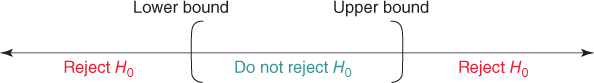
Figure 5.3 Reject values of  that would fall outside the equivalent confidence interval.
- If a certain hypothesized value for
 falls outside the confidence interval with confidence level
  , then the two-tailed hypothesis test with level of significance
  will reject
  for that value of
  .
. - If the hypothesized value for
 falls inside the confidence interval with confidence level
  , then the two-tailed hypothesis test with level of significance
  will not reject
  for that value of
  .
.
For example, recall that our 95% confidence interval for the population mean number of customer service calls for all customers who have the International Plan and the Voice Mail plan and who have more than 220 minutes of day use is
We may use this confidence interval to test any number of possible values of ![]() , as long as the test is two-tailed with level of significance
, as long as the test is two-tailed with level of significance ![]() . For example, use level of significance
. For example, use level of significance ![]() to test whether the mean number of customer service calls for such customers differs from the following values:
to test whether the mean number of customer service calls for such customers differs from the following values:
- 0.5
- 1.0
- 2.4
The solution is as follows. We have the following hypothesis tests:
We construct the 95% confidence interval, and place the hypothesized values of ![]() on the number line, as shown in Figure 5.4.
on the number line, as shown in Figure 5.4.
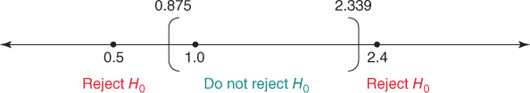
Figure 5.4 Placing the hypothesized values of  on the number line in relation to the confidence interval informs us immediately of the conclusion.
Their placement in relation to the confidence interval allows us to immediately state the conclusion of the two-tailed hypothesis test with level of significance ![]() , as shown in Table 6.6.
, as shown in Table 6.6.
Table 6.6 Conclusions for three hypothesis tests using the confidence interval
| Hypotheses | Position in Relation to 95% | ||
| with |
Confidence Interval | Conclusion | |
| 0.5 | Outside | Reject |
|
| 1.0 | Inside | Do not reject |
|
| 2.4 | Outside | Reject |
5.11 Hypothesis Testing for The Proportion
Hypothesis tests may also be performed about the population proportion ![]() . The test statistic is
. The test statistic is
where ![]() is the hypothesized value of
is the hypothesized value of ![]() , and p is the sample proportion
, and p is the sample proportion
The hypotheses and p-values are shown in Table 6.7.
Table 6.7 Hypotheses and p-values for hypothesis tests about π
| Hypotheses with |
p-Value |
| Left-tailed test. |
|
| Right-tailed test. |
|
| Two-tailed test. |
If If |
For example, recall that 483 of 3333 customers in our sample had churned, so that an estimate of the population proportion ![]() of all of the company's customers who churn is
of all of the company's customers who churn is
Suppose we would like to test using level of significance ![]() whether
whether ![]() differs from 0.15. The hypotheses are
differs from 0.15. The hypotheses are
The test statistic is
As ![]() the p-value =
the p-value = ![]() .
.
As the p-value is not less than ![]() , we would not reject
, we would not reject ![]() . There is insufficient evidence that the proportion of all our customers who churn differs from 15%. Further, assessing the strength of evidence against the null hypothesis using Table 6.5 would lead us to state that there is no evidence against
. There is insufficient evidence that the proportion of all our customers who churn differs from 15%. Further, assessing the strength of evidence against the null hypothesis using Table 6.5 would lead us to state that there is no evidence against ![]() . Also, given a confidence interval, we may perform two-tailed hypothesis tests for
. Also, given a confidence interval, we may perform two-tailed hypothesis tests for ![]() , just as we did for
, just as we did for ![]() .
.
Reference
- Much more information regarding the topics covered in this chapter may be found in any introductory statistics textbook, such as Discovering Statistics, 2nd edition, by Daniel T. Larose, W. H. Freeman, New York, 2013.
R Reference
- R Core Team. R: A Language and Environment for Statistical Computing. Vienna, Austria: R Foundation for Statistical Computing; 2012. ISBN: 3-900051-07-0, http://www.R-project.org/.
Exercises
Clarifying The Concepts
1. Explain what is meant by statistical inference. Give an example of statistical inference from everyday life, say, a political poll.
2. What is the difference between a population and a sample?
3. Describe the difference between a parameter and a statistic.
4. When should statistical inference not be applied?
5. What is the difference between point estimation and confidence interval estimation?
6. Discuss the relationship between the width of a confidence interval and the confidence level associated with it.
7. Discuss the relationship between the sample size and the width of a confidence interval. Which is better, a wide interval or a tight interval? Why?
8. Explain what we mean by sampling error.
9. What is the meaning of the term margin of error?
10. What are the two ways to reduce margin of error, and what is the recommended way?
11. A political poll has a margin of error of 3%. How do we interpret this number?
12. What is hypothesis testing?
13. Describe the two ways a correct conclusion can be made, and the two ways an incorrect conclusion can be made.
14. Explain clearly why a small p-value leads to rejection of the null hypothesis.
15. Explain why it may not always be desirable to draw a black-and-white, up-or-down conclusion in a hypothesis test. What can we do instead?
16. How can we use a confidence interval to conduct hypothesis tests?
Working with the Data
17. The duration customer service calls to an insurance company is normally distributed, with mean 20 minutes, and standard deviation 5 minutes. For the following sample sizes, construct a 95% confidence interval for the population mean duration of customer service calls.
- n = 25
- n = 100
- n = 400.
18. For each of the confidence intervals in the previous exercise, calculate and interpret the margin of error.
19. Refer to the previous exercise. Describe the relationship between margin of error and sample size.
20. Of 1000 customers who received promotional materials for a marketing campaign, 100 responded to the promotion. For the following confidence levels, construct a confidence interval for the population proportion who would respond to the promotion.
- 90%
- 95%
- 99%.
21. For each of the confidence intervals in the previous exercise, calculate and interpret the margin of error.
22. Refer to the previous exercise. Describe the relationship between margin of error and confidence level.
23. A sample of 100 donors to a charity has a mean donation amount of $55 with a sample standard deviation of $25. Test using ![]() whether the population mean donation amount exceeds $50.
whether the population mean donation amount exceeds $50.
- Provide the hypotheses. State the meaning of
 .
. - What is the rejection rule?
- What is the meaning of the test statistic
 ?
? - Is the value of the test statistic
 extreme? How can we tell?
 - What is the meaning of the p-value in this example?
- What is our conclusion?
- Interpret our conclusion so that a nonspecialist could understand it.
24. Refer to the hypothesis test in the previous exercise. Suppose we now set ![]() .
.
- What would our conclusion now be? Interpret this conclusion.
- Note that the conclusion has been reversed simply because we have changed the value of
 . But have the data changed? No, simply our level of what we consider to be significance. Instead, go ahead and assess the strength of evidence against the null hypothesis.
25. Refer to the first confidence interval you calculated for the population mean duration of customer service calls. Use this confidence interval to test whether this population mean differs from the following values, using level of significance ![]() .
.
- 15 minutes
- 20 minutes
- 25 minutes.
26. In a sample of 100 customers, 240 churned when the company raised rates. Test whether the population proportion of churners is less than 25%, using level of significance ![]() .
.