
4
SMC of Markovian Jump Singular Systems with Stochastic Perturbation
4.1 Introduction
In this chapter, we will investigate the SMC design problem for Markovian jump singular systems with stochastic perturbation. The stochastic perturbation considered here is described as a Brownian motion, thus the overall dynamics is actually governed by an Itô stochastic differential equation with Markovian switching parameters and singularity, namely a Markovian jump singular stochastic system. There have been some results reported on SMC of stochastic systems [155, 156, 158] and Markovian jump stochastic systems [157], but the SMC problem for a Markovian jump singular stochastic system has not been fully investigated and still remains challenging. Due to the stochastic perturbation, the stability analysis methods proposed in Chapters 2 and 3 are not fully applicable in this chapter. The commonly used method of analyzing the stability of stochastic systems is based on the Itô formula. In [23], Boukas proposed a sufficient stability condition for a Markovian jump singular stochastic system, but the results are not all of strict LMI form since there exist some matrix equality constraints, which may cause problems in checking the conditions numerically.
We shall design an appropriate integral sliding surface, taking the singular matrix E into account. As a result, the sliding mode dynamics, described by a Markovian jump singular stochastic system, can be easily derived. The order of the resulting sliding mode dynamics is equivalent to that of the original system, which is convenient for analyzing its stochastic stability and the disturbance attenuation performance. A sufficient condition is proposed for the stochastic stability of the sliding mode dynamics in terms of strict LMIs, and by which the sliding surface can be designed. Following this, a discontinuous SMC law is synthesized to force the system state trajectories onto the sliding surface in a finite time. In addition, we also consider the disturbance attenuation problem when there exists an external disturbance in the sliding mode dynamics. A sufficient condition is established, which guarantees the sliding mode dynamics to be stochastically stable with an optimal ![]() performance.
performance.
4.2 System Description and Preliminaries
Consider Markovian jump singular stochastic systems described by
where {rt, t ≥ 0} is a continuous-time Markov process on the probability space which has been defined in (2.2) of Chapter 2; x(t) ∈ Rn is the system state vector; u(t) ∈ Rm is the control input; ϖ(t) is a one-dimensional Brownian motion satisfying E{dϖ(t)} = 0 and E{dϖ2(t)} = dt. Matrix E ∈ Rn × n may be singular, and we assume that rank(E) = r ≤ n. A( · ), B( · ); and D( · ) are known real matrices with appropriate dimensions. f(x, rt) ∈ Rm are unknown nonlinear functions satisfying
where ϵ(rt) > 0 are constant scalars and we define ![]() .
.
For each possible value ![]() , A(rt) = Ai, B(rt) = Bi, D(rt) = Di, and f(x, rt) = fi(x). Then, system (4.1) can be described by
, A(rt) = Ai, B(rt) = Bi, D(rt) = Di, and f(x, rt) = fi(x). Then, system (4.1) can be described by
Assumption 4.1 For each ![]() , the pair (Ai, Bi) in (4.3) is controllable, and the matrix Bi has full column rank.
, the pair (Ai, Bi) in (4.3) is controllable, and the matrix Bi has full column rank.
The nominal system of (4.3) can be formulated as
Definition 4.2.1 The Markovian jump singular stochastic system in (4.4) is said to be stochastically stable if for any x0 ∈ Rn and ![]() , there exists a positive scalar T(x0, r0) such that
, there exists a positive scalar T(x0, r0) such that

We first recall the following lemma [23].
Lemma 4.2.2 The Markovian jump singular stochastic system in (4.4) is stochastically stable if there exist nonsingular matrices Xi, such that for ![]() ,
,

4.3 Integral SMC
4.3.1 Sliding Mode Dynamics Analysis
Design the following integral switching function:

where for each ![]() , Gi ∈ Rm × n and Ki ∈ Rm × n are real matrices to be designed later. The matrix Gi is designed to satisfy that GiBi is nonsingular and GiDi = 0.
, Gi ∈ Rm × n and Ki ∈ Rm × n are real matrices to be designed later. The matrix Gi is designed to satisfy that GiBi is nonsingular and GiDi = 0.
The solution of Ex(t) is given as

It follows from (4.5) and (4.6) that

According to SMC theory, when the system state trajectories reach onto the sliding surface, it follows that s(t) = 0 and ![]() . Then, by
. Then, by ![]() , we obtain the equivalent control law as
, we obtain the equivalent control law as
Thus, by substituting (4.7) into (4.3), the sliding mode dynamics can be obtained as
Now, we will analyze the stability of the sliding mode dynamics in (4.8) based on Lemma 4.2.2.
Proposition 4.3.1 The sliding mode dynamics in (4.8) is stochastically stable if there exist nonsingular matrices Xi such that the following conditions hold for ![]() ,
,

Remark 4.1 Notice that the conditions in Proposition 4.3.1 are not all of strict LMI form owing to the matrix equality constraint of (4.9a). This may cause problems in checking the conditions numerically, since a matrix equality constraint is fragile and usually not satisfied perfectly. Therefore, the strict LMI conditions are more desirable than non-strict ones from the numerical point of view.
In the following, we present a new condition in terms of strict LMIs for the stochastic stability of the sliding mode dynamics in (4.8).
Proposition 4.3.2 The sliding mode dynamics in (4.8) is stochastically stable if there exist matrices Pi > 0 and nonsingular matrices Qi such that for ![]() ,
,

where R ∈ R(n − r) × n and S ∈ Rn × (n − r) are matrices satisfying RE = 0 and ES = 0.
Proof. Letting Xi≜PiE + RTQiST in (4.10), we can obtain (4.9a)–(4.9b). Thus, by Proposition 4.3.1 we know that the sliding mode dynamics in (4.8) is stochastically stable. This completes the proof.
In the following, we present a strict LMI condition for solving parameter Ki in the switching function of (4.5). Before proceeding, we use the following lemma (i.e. Lemma 2.4.3 in Chapter 2) which will play a key role in the sequel.
Lemma 4.3.3 Let Pi be symmetric matrices such that ETLPiEL > 0 and suppose Qi is nonsingular. Then, PiE + RTQiST is nonsingular and
where ![]() are symmetric matrices and
are symmetric matrices and ![]() are nonsingular matrices with
are nonsingular matrices with
Theorem 4.3.4 The sliding mode dynamics in (4.8) is stochastically stable if there exist symmetric matrices ![]() , nonsingular matrices
, nonsingular matrices ![]() , and matrices
, and matrices ![]() ,
, ![]() such that for
such that for ![]() ,
,

where ![]() and
and

Moreover, the parametric matrices Ki in the switching function of (4.5) can be computed by
Proof By Proposition 4.3.2 we know that the sliding mode dynamics in (4.8) is stochastically stable if there exist matrices Pi > 0 and nonsingular matrices Qi, such that the conditions of (4.10) hold for ![]() . Moreover, according to Lemma 4.3.3, we know that PiE + RTQiST are nonsingular and
. Moreover, according to Lemma 4.3.3, we know that PiE + RTQiST are nonsingular and ![]() . Now, performing a congruence transformation on (4.10) by matrices
. Now, performing a congruence transformation on (4.10) by matrices ![]() , we have
, we have
Letting ![]() and
and ![]() , we have
, we have
But the following fact is true:

Considering πii < 0, thus we have
Therefore, (4.13) holds if the following inequalities hold for ![]() :
:

By Schur complement, (4.14) is equivalent to (4.11). This completes the proof. ▀
4.3.2 SMC Law Design
In the following, we shall design an SMC law, by which the state trajectories of the Markovian jump singular stochastic system in (4.1) can be driven onto the designed sliding surface s(t) = 0 in a finite time and maintained there for all subsequent time.
Theorem 4.3.5 Consider the Markovian jump singular stochastic system in (4.1). Suppose that the switching function is given as (4.5) with Ki being solved by (4.12), and Gi is chosen to satisfy that GiBi is nonsingular and GiDi = 0. Then, the state trajectories of system (4.1) can be driven onto the sliding surface s(t) = 0 by the following SMC law:
where λ > 0 is an adjustable scalar.
Proof We choose Gi as Gi = BTiYi, where Yi > 0 are matrices to be designed such that GiBi = BTiYiBi > 0 for ![]() . Choose the following Lyapunov function:
. Choose the following Lyapunov function:
According to (4.5), we have

Substituting (4.15) into (4.16) yields
Thus, taking the derivation of V(t) and considering (4.17), we have

which implies that the state trajectories of the system in (4.1) will be driven onto the sliding surface s(t) = 0 in a finite time. This completes the proof.
In the implementation of the SMC law in (4.15), the upper bound scalar ϵ of fi(t) in (4.2) is required to be known a priori. If the value of ϵ is not available, we have to estimate it. In the following theorem, we shall consider this case, and first design an adaptive law to estimate ϵ, thus an adaptive SMC law will be presented for system (4.1).
Theorem 4.3.6 Consider the Markovian jump singular stochastic system in (4.1), and assume that the exact value of the upper bound scalar ϵ is not available. Suppose that the switching function is given as (4.5) with Ki being solved by (4.12), and Gi is chosen to satisfy that GiBi are nonsingular and GiDi = 0. Then, the state trajectories of system (4.1) can be driven onto the sliding surface s(t) = 0 by the following adaptive SMC law:
where ![]() represents the estimate of ϵ, and the adaptive law is given as
represents the estimate of ϵ, and the adaptive law is given as
with ϵ(0) = 0, where δ > 0 is an adjustable scalar.
Proof Select the following Lyapunov function:
The rest of the proof can be followed along the same lines as the proof of Theorem 4.3.5. ▀
4.4 Optimal  Integral SMC
In this section, within the framework of the SMC problem, we shall further analyze the ![]() performance for Markovian jump singular stochastic systems with an
performance for Markovian jump singular stochastic systems with an ![]() external disturbance. Specifically, we will propose a sufficient condition by which the sliding mode dynamics of the controlled system is guaranteed to be stochastically stable with an
external disturbance. Specifically, we will propose a sufficient condition by which the sliding mode dynamics of the controlled system is guaranteed to be stochastically stable with an ![]() performance.
performance.
4.4.1 Performance Analysis and SMC Law Design
Consider the following singular stochastic systems with Markovian jump parameters and an external disturbance:
where ω(t) ∈ Rp is the disturbance input which belongs to ![]() ; z(t) ∈ Rq is the controlled output; Ci, Fi and Hi are real constant matrices. Unless other specified, the notations in (4.18a)–(4.18b) have the same meanings as those in (4.1).
; z(t) ∈ Rq is the controlled output; Ci, Fi and Hi are real constant matrices. Unless other specified, the notations in (4.18a)–(4.18b) have the same meanings as those in (4.1).
Designing the same switching function as in (4.5) and employing the methods used in Section 4.3, we can obtain the following sliding mode dynamics:
Remark 4.2 Notice from (4.19) that if matrix Fi in (4.18a)–(4.18b) satisfies the so-called matching condition – that is, there exist matrices ![]() satisfying
satisfying ![]() – it follows that the sliding mode dynamics in (4.19) becomes (4.8). This implies that the sliding mode dynamics is adaptive to the disturbance ω(t). In this case, the methods proposed in the previous section of this chapter can be applied directly. In the following, we assume that matrix Fi does not satisfy the matching condition, thus there will exist a disturbance ω(t) in the sliding mode dynamics, and the results will be sharply different from the matching case.
– it follows that the sliding mode dynamics in (4.19) becomes (4.8). This implies that the sliding mode dynamics is adaptive to the disturbance ω(t). In this case, the methods proposed in the previous section of this chapter can be applied directly. In the following, we assume that matrix Fi does not satisfy the matching condition, thus there will exist a disturbance ω(t) in the sliding mode dynamics, and the results will be sharply different from the matching case.
Definition 4.4.1 Given a scalar γ > 0, the sliding mode dynamics in (4.19) is said to be stochastically stable with an ![]() performance level γ, if it is stochastically stable with ω(t) = 0, and under zero condition, for nonzero
performance level γ, if it is stochastically stable with ω(t) = 0, and under zero condition, for nonzero ![]() , it holds that
, it holds that

Now, we will analyze the stability and the ![]() performance of the sliding mode dynamics in (4.19).
performance of the sliding mode dynamics in (4.19).
Theorem 4.4.2 Given a scalar γ > 0, the sliding mode dynamics in (4.19) is stochastically stable with an ![]() performance level γ, if there exist nonsingular matrices
performance level γ, if there exist nonsingular matrices ![]() such that for
such that for ![]() ,
,

where

Proof Choose the following Lyapunov function:
where ![]() and
and ![]() (denoted by
(denoted by ![]() when rt = i) are nonsingular matrices to be specified such that
when rt = i) are nonsingular matrices to be specified such that ![]() are positive definite for
are positive definite for ![]() .
.
Let ![]() be the infinitesimal generator of the Markov process {(x(t), rt), t ≥ 0}. Then, the average derivative emanating from point (x, i) at time t is given by the following expression:
be the infinitesimal generator of the Markov process {(x(t), rt), t ≥ 0}. Then, the average derivative emanating from point (x, i) at time t is given by the following expression:

where

Here, we choose ![]() in the above derivation, which guarantees that
in the above derivation, which guarantees that ![]() is nonsingular since
is nonsingular since ![]() . In addition,
. In addition, ![]() are introduced due to GiDi = 0. Therefore, when ω(t) = 0 in (4.22), it follows that
are introduced due to GiDi = 0. Therefore, when ω(t) = 0 in (4.22), it follows that ![]() . By Schur complement, (4.21b) implies ϒi < 0 for
. By Schur complement, (4.21b) implies ϒi < 0 for ![]() , thus,
, thus,
Therefore, we know that the the sliding mode dynamics in (4.19) with ω(t) = 0 is stochastically stable.
Now, we will establish the ![]() performance. To this end, assume zero initial condition (that is, x(0) = 0, thus W(0, r0) = 0) and consider index:
performance. To this end, assume zero initial condition (that is, x(0) = 0, thus W(0, r0) = 0) and consider index:

Dynkin’s formula gives

and together with (4.22), we have

where Ξ12i and Ξ22i are defined in (4.21b). By Schur complement, (4.21b) implies

Then ![]() from (4.23), thus (4.20) holds. This completes the proof. ▀
from (4.23), thus (4.20) holds. This completes the proof. ▀
The following theorem will give a sufficient condition by which the sliding mode dynamics in (4.19) is guaranteed to be stochastically stable with an ![]() performance level γ, and the switching function in (4.5) can be solved.
performance level γ, and the switching function in (4.5) can be solved.
Theorem 4.4.3 Given a scalar γ > 0, the sliding mode dynamics in (4.19) is stochastically stable with an ![]() performance level γ, if there exist symmetric matrices
performance level γ, if there exist symmetric matrices ![]() , positive definite matrices
, positive definite matrices ![]() ,
, ![]() , nonsingular matrices
, nonsingular matrices ![]() , and matrices
, and matrices ![]() ,
, ![]() such that for
such that for ![]() ,
,

where

Moreover, the parametric matrices Ki in the switching function of (4.5) can be computed by

Proof From Proposition 4.3.2, it can be seen that the sliding mode dynamics in (4.19) is stochastically stable with an ![]() performance level γ, if there exist matrices Pi > 0 and nonsingular matrices Qi such that for
performance level γ, if there exist matrices Pi > 0 and nonsingular matrices Qi such that for ![]() ,
,

where

By Lemma 4.3.3, we know that Zi≜PiE + RTQiST are nonsingular and ![]() , where
, where ![]() are symmetric matrices and
are symmetric matrices and ![]() are nonsingular matrices with
are nonsingular matrices with
Now, performing a congruence transformation on (4.26) by ![]() , we have
, we have

where ![]() are defined in (4.24a) and
are defined in (4.24a) and

Notice that
Letting ![]() and
and ![]() , we know that (4.28) holds if for
, we know that (4.28) holds if for ![]() ,
,

where
where ![]() , and the other notations are defined in (4.24a). Furthermore, considering (4.24b) and (4.24d), inequality (4.24a) yields (4.29), and (4.24c) yields (4.27). This completes the proof. ▀
, and the other notations are defined in (4.24a). Furthermore, considering (4.24b) and (4.24d), inequality (4.24a) yields (4.29), and (4.24c) yields (4.27). This completes the proof. ▀
Now, by applying the same procedures as in Section 4.3, we design a discontinuous SMC law to drive the system state trajectories onto the predefined sliding surface in a finite time and maintain it there for all the subsequent time.
Theorem 4.4.4 Consider the Markovian jump singular stochastic system in (4.1). Suppose that the switching function is given as (4.5) with Ki being solved by (4.25), and Gi are chosen as ![]() , where
, where ![]() is the solution of (4.24a)–(4.24d). Then, the state trajectories of system (4.1) can be driven onto the sliding surface s(t) = 0 by the SMC law u(t) designed in (4.15).
is the solution of (4.24a)–(4.24d). Then, the state trajectories of system (4.1) can be driven onto the sliding surface s(t) = 0 by the SMC law u(t) designed in (4.15).
4.4.2 Computational Algorithm
Notice that there exist three matrix equalities of (4.24b)–(4.24d) in Theorem 4.4.3, which can not be solved directly by applying the LMI procedures. In the following, we will propose some algorithms to solve them. Firstly, to solve (4.24b)–(4.24c), we consider the following matrix inequalities for scalars α > 0 and β > 0,
By Schur complement, (4.30) and (4.31) are respectively equivalent to

Therefore, when α > 0 and β > 0 are chosen as two sufficiently small scalars, matrix equalities (4.24b) and (4.24c) can be solved through LMIs (4.32) and (4.33), respectively.
We use the CCL method [66] to solve (4.24d) by formulating it into a sequential optimization problem subject to LMI constraints. We suggest the following minimization problem involving LMI conditions instead of the original nonconvex feasibility problem in Theorem 4.4.3.
Problem SMDA (Sliding mode dynamics analysis):

If the solution of the aforesaid minimization problem is Nr, then the conditions in Theorem 4.4.3 are solvable. Although it is still not possible to always find the global optimal solution, the proposed minimization problem is easier to solve than the original nonconvex feasibility problem. We suggest the following algorithm to solve Problem SMDA.
Algorithm SMDA
- Step 1. Choose α > 0 and β > 0 as sufficiently small scalars.
- Step 2. Find a feasible set
 satisfying (4.24a), (4.32)–(4.33), and (4.34). Set κ = 0.
 - Step 3. Solve the following optimization problem
and denote f* as the optimized value.

- Step 4. Substitute the obtained matrices
 into (4.29). If (4.29) is satisfied, with
for a sufficiently small scalar ϵ > 0, then output the feasible solutions
into (4.29). If (4.29) is satisfied, with
for a sufficiently small scalar ϵ > 0, then output the feasible solutions
 , so EXIT.
 - Step 5. If
 where
where  is the maximum number of iterations allowed, so EXIT.
 - Step 6. Set κ = κ + 1,
 , and go to Step 3.
4.5 Illustrative Example
Example 4.5.1 Consider the Markovian jump singular stochastic system in (4.1) with two operating modes, that is, N = 2 and the following parameters:
In addition, f1(x) = f2(x) = 1.5exp ( − t)sin (t)x(t) (thus, ϵ in (4.2) can be chosen as ϵ = 1.5) and
Here, we only simulate the results in Section 4.3. Our aim is to design an SMC law u(t) in (4.15) such that the closed-loop system is stochastically stable. Solving the LMI conditions in Theorem 4.3.4, we obtain

Thus, by (4.12) we have
Here, parameter Gi, i ∈ {1, 2} in (4.5) can be chosen as ![]() . Thus, GiBi are nonsingular and GiDi = 0 are guaranteed for i ∈ {1, 2}. By (4.5), the switching functions can be computed as
. Thus, GiBi are nonsingular and GiDi = 0 are guaranteed for i ∈ {1, 2}. By (4.5), the switching functions can be computed as

Let the adjustable scalar λ be λ = 0.5, then the SMC law designed in (4.15) can be computed as

To prevent the control signals from chattering, we replace sign(s(t)) with ![]() . By using the discretization approach [96], we simulate standard Brownian motion. Some initial parameters are given as follows: the simulation time t ∈ [0, T*] with T* = 8, the normally distributed variance
. By using the discretization approach [96], we simulate standard Brownian motion. Some initial parameters are given as follows: the simulation time t ∈ [0, T*] with T* = 8, the normally distributed variance ![]() with N* = 211, step size Δt = ρδt with ρ = 2, and the number of discretized Brownian paths p = 10. The simulation results are given in Figures 4.1–4.7. Among them, Figures 4.1–4.3 are the simulation results along an individual discretized Brownian path. Figure 4.1 shows the states of the closed-loop system; Figure 4.2 depicts the switching function s(t); and Figure 4.3 gives the SMC input u(t). Figures 4.4–4.7 show the corresponding simulation results along 10 individual paths (dotted lines) and the average over 10 paths (solid line). Figures 4.4–4.6 show the states of the closed-loop system. Figure 4.7 depicts the switching function s(t).
with N* = 211, step size Δt = ρδt with ρ = 2, and the number of discretized Brownian paths p = 10. The simulation results are given in Figures 4.1–4.7. Among them, Figures 4.1–4.3 are the simulation results along an individual discretized Brownian path. Figure 4.1 shows the states of the closed-loop system; Figure 4.2 depicts the switching function s(t); and Figure 4.3 gives the SMC input u(t). Figures 4.4–4.7 show the corresponding simulation results along 10 individual paths (dotted lines) and the average over 10 paths (solid line). Figures 4.4–4.6 show the states of the closed-loop system. Figure 4.7 depicts the switching function s(t).

Figure 4.1 States of the closed-loop system
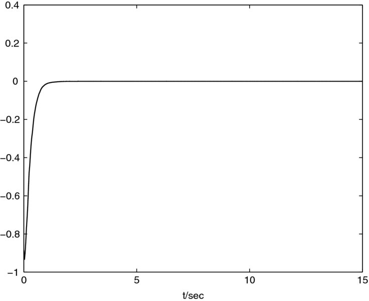
Figure 4.2 Switching function

Figure 4.3 Control input
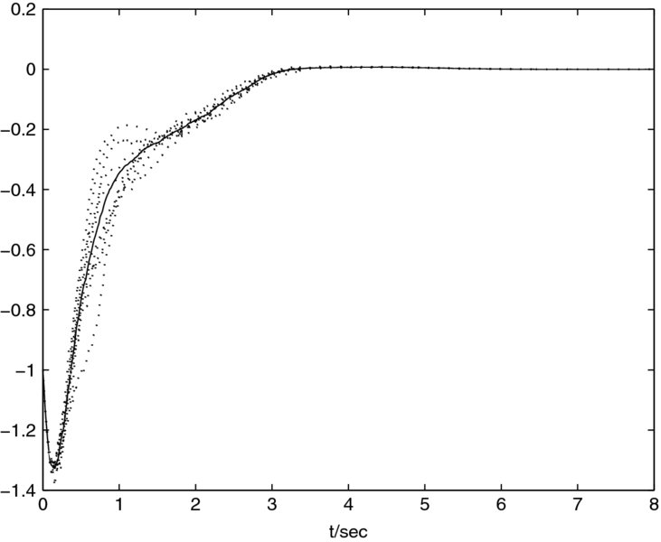
Figure 4.4 Individual paths and the average of the state of the closed-loop system: first component

Figure 4.5 Individual paths and the average of the state of the closed-loop system: second component

Figure 4.6 Individual paths and the average of the state of the closed-loop system: third component

Figure 4.7 Individual paths and the average of the switching function
4.6 Conclusion
In this chapter, SMC of Markovian jump singular stochastic hybrid systems has been investigated. An integral sliding surface has been designed and some sufficient conditions have been proposed for the stochastic stability of sliding mode dynamics in terms of strict LMI. Also, an explicit parametrization of the desired sliding surface has been given. A sliding mode controller has been synthesized to guarantee the reachability of the system state trajectories to the sliding surface. Moreover, we have further analyzed the stochastic stability and ![]() disturbance attenuation performance for the sliding mode dynamics, and some related sufficient conditions have also been proposed. A numerical example has been provided to illustrate the effectiveness of the proposed design scheme.
disturbance attenuation performance for the sliding mode dynamics, and some related sufficient conditions have also been proposed. A numerical example has been provided to illustrate the effectiveness of the proposed design scheme.