
Chapter 12
Autodesk Maya Dynamics and Effects
Special effects animations simulate not only physical phenomena, such as smoke and fire, but also the natural movements of colliding bodies. Behind the latter type of animation is the Autodesk® Maya® dynamics engine, which is the sophisticated software that creates realistic-looking motion based on the principles of physics.
Another Maya animation tool, Paint Effects, can create dynamic fields of grass and flowers, a head full of hair, and other such systems in a matter of minutes. Maya also offers dynamic simulations for hair, fur, and cloth. In this chapter, I’ll cover the basics of dynamics in Maya and let you practice working with particles by making steam.
- Create rigid body dynamic objects and create forces to act upon them
- Keyframe animated passive rigid body objects to act on active rigid bodies
- Bake out simulations to keyframes and simplify animation curves
- Understand nParticle workflow
- Emit nParticles and have them move and render to simulate steam
- Draw Paint Effects strokes
- Render an object with a cartoon look easily
- Create an nCloth object (a.k.a. nMesh)
- Collide nMesh objects and add forces
- Cache your nDynamics to disk
- Customize the Maya interface
An Overview of Dynamics and Maya Nucleus
Dynamics is the simulation of motion through the application of the principles of physics. Rather than assigning keyframes to objects to animate them, with Maya dynamics you assign physical characteristics that define how an object behaves in a simulated world. You create the objects as usual in Maya, and then you convert them to dynamic bodies. Dynamic bodies are defined through dynamic attributes you add to them, which affect how the objects behave in a dynamic simulation.
Dynamic bodies are affected by external forces called fields, which exert a force on them to create motion. Fields can range from wind forces to gravity and can have their own specific effects on dynamic bodies.
In Maya, dynamic objects are categorized as bodies, particles, hair, and fluids. Dynamic bodies are created from geometric surfaces and are used for physical objects such as bouncing balls. Particles are points in space that have renderable properties and are used for numerous effects, such as fire and smoke. I’ll cover particle basics in the latter half of this chapter. Hair consists of curves that behave dynamically, such as strings. Fluids are, in essence, volumetric particles that can exhibit surface properties. You can use fluid dynamics for natural effects such as billowing clouds or plumes of smoke.
Nucleus is a more stable and interactive way of calculating dynamic simulations in Maya than its traditional dynamics engine. Nucleus speeds up the creation and increases the stability of some dynamic effects in Maya, including particle effects and cloth simulation (through nCloth).
In the Maya 2009 release, Autodesk introduced nParticles. They’re closely related to traditional particles in Maya but have been made easier to create and manage, requiring less-explicit expression controls than before.
I’ll introduce nParticles (instead of traditional particles) later in this chapter; however, soft bodies, hair, nCloth, and fluid dynamics are advanced topics and won’t be covered in this book.
Rigid and Soft Dynamic Bodies
The two types of dynamic bodies are rigid and soft. Rigid bodies are solid objects, such as a pair of dice or a baseball, that move and rotate according to the dynamics applied. Fields and collisions affect the entire object and move it accordingly. Soft bodies are malleable surfaces that deform dynamically, such as drapes in the wind or a bouncing rubber ball. In brief, this is accomplished by making the surface points (NURBS, CVs, or polygon vertices) of the soft body object dynamic instead of the whole object. The forces and collisions of the scene affect these surface points, making them move to deform their surface. In this section, you’ll learn about rigid body dynamics.
Creating Active and Passive Rigid Body Objects
Any surface geometry in Maya can be converted to a rigid body. After it’s converted, that surface can respond to the effects of fields and take part in collisions. Sounds like fun, eh?
The two types of rigid bodies are active and passive. An active rigid body is affected by collisions and fields. A passive rigid body isn’t affected by fields and remains still when it collides with another object. A passive rigid body is used as a surface against which active rigid bodies collide.
The best way to see how the two types of rigid bodies behave is to create some and animate them. In this section, you’ll do that in the classic animation exercise of a bouncing ball.
To create a bouncing ball using Maya rigid bodies, switch to the Dynamics menu and follow these steps:
Figure 12-1: Place a poly sphere a few units above a poly plane ground surface.

To play back the simulation, set your frame range from 1 to at least 500. Go to frame 1, and click Play. Make sure you have the proper Playback Speed settings in your Preferences window; otherwise, the simulation won’t play properly.
When the simulation plays, you’ll notice that the sphere begins to fall after a few frames and collides with the ground plane, bouncing back up.
As an experiment, try turning the passive body plane into an active body using the following steps:
To connect the now-active body plane to the gravity field, open the Dynamic Relationships Editor window, shown in Figure 12-2 (choose Window ⇒ Relationship Editors ⇒ Dynamic Relationships).
Figure 12-2: The Dynamic Relationships Editor window

On the left is an Outliner list of the objects in your scene. On the right is a list from which you can choose a category of objects to list: Fields (default), Collisions, Emitters, or All. Select the geometry (pPlane1) on the left side, and then connect it to the gravity field by selecting the gravityField1 node on the right.
When you connect the gravity field to the plane and run the simulation, you’ll see the plane fall away with the ball. Because the two fall at the same rate (the rate set by the single gravity field), they don’t collide. To disconnect the plane from the gravity field, deselect the gravity field in the right panel.
Turning the active body plane back to a passive floor is as simple as returning to frame 1, the beginning of the simulation, and clearing the Active attribute in the Attribute Editor. By turning the active body back to a passive body, you regain an immovable floor upon which the ball can collide and bounce.
Moving a Rigid Body
Because the Maya dynamics engine controls the movement of any active rigid bodies, you can’t set keyframes on their translation or rotation. With a passive object, however, you can set keyframes on translation and rotation as you can with any other Maya object. You also can easily keyframe an object to turn either active or passive.
Any movement that the passive body has through regular keyframe animation is translated into momentum, which is passed on to any active rigid bodies with which the passive body collides. Think of a baseball bat that strikes a baseball. The bat is a passive rigid body that you have keyframed to swing. The baseball is an active rigid body that is hit by (collides with) the bat as it swings. The momentum of the bat is transferred to the ball, and the ball is sent flying into the stadium stands. You’ll see an example of this in action in the next exercise.
Rigid Body Attributes
Here is a rundown of the more important attributes for both passive and active rigid bodies as they pertain to collisions:
Animating with Dynamics: The Pool Table
This exercise will take you through the creation of a scene in which you’ll use dynamics to animate a cue ball striking two balls on a pool table.
Creating the Pool Table and the Balls
You’ll create a simple pool table as a collision surface for the pool balls. To create the table, follow these steps:
Figure 12-3: Duplicate the tabletop plane, and offset it slightly in both directions.

Figure 12-4: A simple pool table

Figure 12-5: Scaling and placing the three spheres
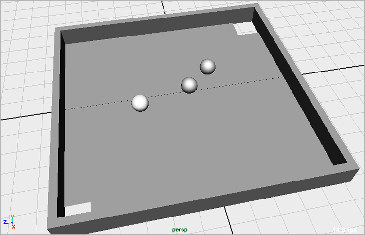
Figure 12-6: The pool balls in texture view

The spheres are placed a bit over the table surface so that their geometries’ surfaces aren’t accidentally crossing each other, an effect known as interpenetrating. When surfaces interpenetrate, the dynamics that result are usually as welcome as sand in your eyes. Starting all colliding rigid bodies slightly away from each other should guarantee that their surfaces don’t interpenetrate. Using the simple pool table that you’ve set up will make the dynamics calculations quick and easy.
Use the file Table_v1.mb in the Scenes folder of the Pool_Table project on the book’s companion web page, www.sybex.com/go/introducingmaya2014, as a reference or to catch up to this point.
Creating Rigid Bodies
Define the pool table as a passive rigid body, and define the pool balls as active rigid bodies. Follow these steps:
Animating Rigid Bodies
If you need to, enable texture view in your view panel by pressing 6.
The next step is to put the cue ball (the white sphere) into motion so that it hits the striped ball into the black eight ball to sink it into the corner pocket. Keyframe the cue ball’s translation from its starting point to hit into the striped ball. However, because active rigid bodies can’t be keyframed, you have to turn the cue ball into a passive rigid body. To do that, follow these steps:
Figure 12-7: Move the cue ball with the Translate tool.

By animating the ball as a passive rigid body, keyframing its translation, and then turning it back to active, you set the dynamic simulation in motion. The cue ball animates from its starting position and hits the striped ball. The Maya dynamics engine calculates the collisions on that ball and sets it into motion; the ball then strikes the black eight ball, which should roll into the corner pocket. The dynamics engine, at frame 11, also calculates the movement of the cue ball after it strikes the striped ball, so you don’t have to animate its ricochet.
Go to the start frame, and play back the simulation. The cue ball knocks the striped ball into the eight ball. The eight ball rolls into the corner, and the striped ball bounces off to the right. If the eight ball doesn’t go into the corner, you’ll have to edit your cue ball’s keyframes to hit the striped ball at the correct angle to hit the eight ball into the corner pocket.
At the current settings, however, the eight ball bounces out of the corner without falling through the hole. You need to control the bounciness of the collisions.
Figure 12-8: The eight ball falls through the hole.

You can download the scene file Table_v2.mb from the Pool_Table project on the web page to compare your work.
Additional Rigid Body Attributes
In addition, while using the pool table setup without any animation, try playing with the rigid body attributes to see how they affect the rigid body in question. Some of these attributes are defined here:
Creating animation with rigid bodies is straightforward and can go a long way toward creating natural-looking motion for your scene. Integrating such animation into a final project can become fairly complicated, though, so it’s prudent to become familiar with the workings of rigid body dynamics before relying on that sort of workflow for an animated project. You’ll find that most professionals use rigid body dynamics as a springboard to create realistic motion for their projects. The dynamics are often converted to keyframes and further tweaked by the animator to fit into a larger scene.
Here are a few suggestions for scenes using rigid body dynamics:
Baking Out a Simulation
Frequently, a dynamic simulation is created to fit into another scene, perhaps to interact with other objects. In instances such as this, you want to exchange the dynamic properties of the dynamic body you have set up in a simulation for regular, good old-fashioned animation curves that you can edit along with the rest of the animated scene, if need be. You can easily take a simulation that you’ve created and bake it out to curves. As much fun as it is to think of cupcakes, baking is a somewhat catchall term used to describe converting one type of action or procedure into another; in this case, you’re baking dynamics into keyframes.
You’ll take the simulation you set up earlier with the pool balls and turn them into keyframes, to give you a quick idea of how it can be done and the curves you’ll get. Dynamics is a deep layer of Maya, and there is a lot to learn about it. Keep in mind that you can use this introduction as a foundation for your own explorations.
To bake out the rigid body simulation of the pool balls, follow these steps:
Figure 12-9: The Bake Simulation Options window
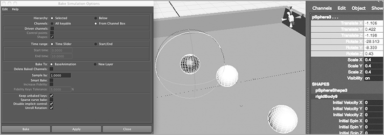
Figure 12-10: The pool balls have animation curves.

Figure 12-11: Sampling by fives makes a cleaner curve.

Sampling by fives may give you an easier curve to edit, but it can oversimplify the animation of your objects; make sure you use the best Sampling setting for your simulation when you need to convert it to curves for editing.
Simplifying Animation Curves
Despite a higher Sampling setting when you bake out the simulation, you can still be left with a lot of keyframes to deal with, especially if you have to modify the animation extensively from here. One last trick you can use is to simplify the curve further through the Graph Editor. You have to work with curves of the same relative size, so you’ll start with the rotation curves, because they have larger values. To keep things simple, let’s deal with one ball: the black eight ball. To simplify the curve in the Graph Editor, follow these steps:
Figure 12-12: The Graph Editor displays the rotation curves of the eight ball.

Figure 12-13: Select the curves to simplify them.

Figure 12-14: A simplified curve for the rotations of the eight ball

Simplifying curves is a handy way to convert a dynamic simulation to curves. Keep in mind that you may lose fidelity to the original animation after you simplify a curve, so use this technique with care. The curve simplification works with good old-fashioned keyframed curves as well; if you inherit a scene from another animator and need to simplify the curves, do it just as you did here.
Fun Dynamics: Shoot the Catapult!
Now for a fun, quick exercise, you’ll use Rigid Body Dynamics to shoot a projectile with the already animated catapult from Chapter 8. Open the scene file catapult_anim_v2.mb from the Catapult_Anim project downloaded from the companion website.
Figure 12-15: Place a sphere over the basket.

Figure 12-16: It puts the sphere in the basket, or else it gets the hose again.

Figure 12-17: Select the vertex.

Figure 12-18: The bowl snaps to the arm at a weird angle.

Figure 12-19: Set offsets to place the bowl properly inside the basket.

Figure 12-20: The ball shoots!

If you play back the scene frame by frame, you’ll notice that the arm and basket will briefly pass through the projectile ball for a few frames as the arm shoots back up around frames 102–104. Increasing the subdivisions of the ball and the bowl before making them rigid bodies will help the collisions, but for a fun exercise, this works great. Play with the placement of the ball at the start of the scene, as well as the gravity and any other fields you care to experiment with to try to land the projectile in different places in the scene.
nParticle Dynamics
Like rigid body objects, particles are moved dynamically using collisions and fields. In short, a particle is a point in space that is given renderable properties—that is, it can render out. When particles are used en masse, they can create effects such as smoke, a swarm of insects, fireworks, and so on. nParticles are an implementation of particles through the Maya Nucleus solver, which provides better and easier simulations than traditional Maya particles.
Although particles (and nParticles) can be an advanced and involved aspect of Maya, it’s important to have some exposure to them as you begin to learn Maya.
Much of what you learned about rigid body dynamics transfers to particles. However, it’s important to think of particle animation as manipulating a larger system rather than as controlling every single particle in the simulation. Particles are most often used together in large numbers so that the entirety is rendered out to create an effect. You control fields and dynamic attributes to govern the motion of the system as a whole.
Emitting nParticles
A typical workflow for creating an nParticle effect in Maya breaks out into two parts: motion and rendering. First, you create and define the behavior of particles through emission. An emitter is a Maya object that creates the particles. After you create fields and adjust particle behavior within a dynamic simulation, much as you would do with rigid body motion, you give the particles renderable qualities to define how they look. This second aspect of the workflow defines how the particles come together to create the desired effect, such as steam. You’ll make a locomotive pump steam later in this chapter.
To create an nParticle system, follow these steps:
Figure 12-21: Creation options for an nParticle emitter

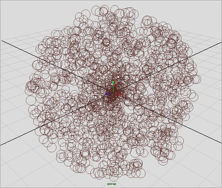
You’ll notice a mass of circles streaming out of the emitter in all directions (see Figure 12-22). These are the nParticles.
Figure 12-22: An Omni emitter emits a swarm of cloud particles in all directions.
Emitter Attributes
You can control how particles are created and behave by changing the type of emitter and adjusting its attributes. Here are the most often used emitters:
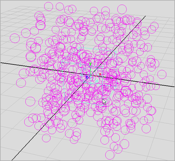
Figure 12-23: Cloud nParticles are sprayed in a specific direction.

Figure 12-24: Cloud nParticles emit from anywhere inside the emitter’s volume.
After you create an emitter, its attributes govern how the particles are released into the scene. Every emitter has the following attributes to control the emission:
Figure 12-25: An emitter with Min and Max Distance settings of 3 emits cloud nParticles 3 units from itself.

nParticle Attributes
After being created, or born, and set into motion by an emitter, nParticles rely on their own attributes and any fields or collisions in the scene to govern their motion, just like rigid body objects.
In Figure 12-26, the Attribute Editor shows a number of tabs for the selected particle object. nParticle1 is the particle object node. This has the familiar Translate, Rotate, and Scale attributes, like most other object nodes. But the shape node, nParticleShape1, is where all the important attributes are for a particle, and it’s displayed by default when you select a particle object. The third tab in the Attribute Editor is the emitter1 node that belongs to the particle’s emitter. This makes it easier to toggle back and forth to adjust emitter and particle settings.
Figure 12-26: nParticle attributes

The Lifespan Attributes
When any particle is born, you can give it a lifespan, which allows the particle to die when it reaches a certain point in time. As you’ll see with the steam locomotive later in the chapter, a particle that has a lifespan can change over that lifespan. For example, a particle may start out as white and fade away at the end of its life. A lifespan also helps keep the total number of particles in a scene to a minimum, which helps the scene run more efficiently.
You use the Lifespan mode to select the type of lifespan for the nParticle.
The Shading Attributes
The Shading attributes determine how your particles look and how they will render. Two types of particle rendering are used in Maya: software and hardware. Hardware particles are typically rendered out separately from anything else in the scene and are then composited with the rest of the scene. Because of this compound workflow for hardware particles, this book will introduce you to a software particle type called Cloud. Cloud, like other software particles, can be rendered with the rest of a scene through the software renderer.
With your particles selected, open the Attribute Editor. In the Shading section, you’ll find the Particle Render Type drop-down menu (see Figure 12-27).
Figure 12-27: The Particle Render Type drop-down menu

The three render types listed with the (s/w) suffix are software-rendered particles. All the other types can be rendered only through the Maya Hardware renderer. Select your render type, and Maya adds the proper attributes you’ll need for the render type you selected.
For example, if you select the Points render type from the menu, your particles change from circles on the screen to dots, as shown in Figure 12-28.
Figure 12-28: Dots on the screen represent point particles.

Several new attributes that control the look of the particles appear when you switch the Particle Render Type setting. Each Particle Render Type setting has its own set of render attributes. Set your nParticles back to the Cloud type. The Cloud particle type attributes are Threshold, Surface Shading, and Opacity. (See Figure 12-29.)
Figure 12-29: Each Particle Render Type setting displays its own set of attributes.

In the Shading heading, shown in Figure 12-30 for the cloud nParticles, are controls for the Opacity Scale, Color, and Incandescence attributes. They control how the particles look when simulated and rendered. Notice how each of these controls is based on ramps.
Figure 12-30: Controls for the Opacity Scale, Color, and Incandescence attributes

nParticles are already set up to allow you to control the color, opacity, and incandescence during the life of the particle. For example, by default, the Color attribute is set up with a white to cyan ramp. This means that each of the particles will begin life white in color and will gradually turn cyan toward the end of its lifespan, or Age setting.
Likewise, the Particle Size heading in the Attribute Editor contains a ramp for Radius Scale that works much the same way as the Color attribute just described. In this case, you use the Radius Scale ramp to increase or decrease the size of the particle along its Age setting.
nCaching Particles
It would be nice to turn particles into cash, but I can only show you how to turn your particles into a cache. You can cache the motion of your particles to memory or to disk to make playback and editing of your particle animation easier. To cache particles to your system’s fast RAM memory, select the nParticle object you want to cache, and open the Attribute Editor. In the Caching section, under Memory Caching, select the Cache Data check box. Play back your scene, and the particles cache into your memory for faster playback. You can also scrub your timeline to see your particle animation. If you make changes to your animation, the scene won’t reflect the changes until you delete the cache from memory by selecting the particle object and unchecking the Memory Cache check box in the Attribute Editor. The amount of information the memory cache can hold depends on your machine’s RAM.
Although memory caching is generally faster than disk caching, creating a disk cache lets you cache all the particles as they exist throughout their duration in your scene and ensures that the particles are rendered correctly, especially if you’re rendering on multiple computers or across a network. You should create a particle disk cache before rendering.
Creating an nCache on Disk
After you’ve created a particle scene and you want to be able to scrub the timeline back and forth to see your particle motion and how it acts in the scene, you can create a particle nCache to disk. This lets you play back the entire scene as you like, without running the simulation from the start and by every frame.
To create an nCache, switch to the nDynamics menu, select the nParticle object, and choose nCache ⇒ Create New Cache. Maya will run the simulation according to the timeline and save the position of all the particle systems in the scene to cache files in your current project’s Data/Cache folder. You can then play or even scrub your animation back and forth, and the particles will run properly.
If you make any dynamics changes to the particles, such as emission rate or speed, you’ll need to detach the cache file from the scene for the changes to take effect. Choose nCache ⇒ Delete Cache. You can open the option box to select whether you want to delete the cache files physically or merely detach them from the current nParticles.
Now that you understand the basics of particle dynamics, it’s time to see for yourself how they work.
Animating a Particle Effect: Locomotive Steam
You’ll create a spray of steam puffing out of the pump on the side of the locomotive that drives the wheels that you rigged previously. You’ll use the scene fancy_locomotive_anim_v3.mb from Chapter 9, “More Animation!”
Emitting the nParticles
The first step is to create an emitter to spray from the steam pump and to set up the motion and behavior of the nParticles.
Figure 12-31: Place the emitter at the end of the pump.

Figure 12-32: Cloud nParticles emit in a straight line from the pump.
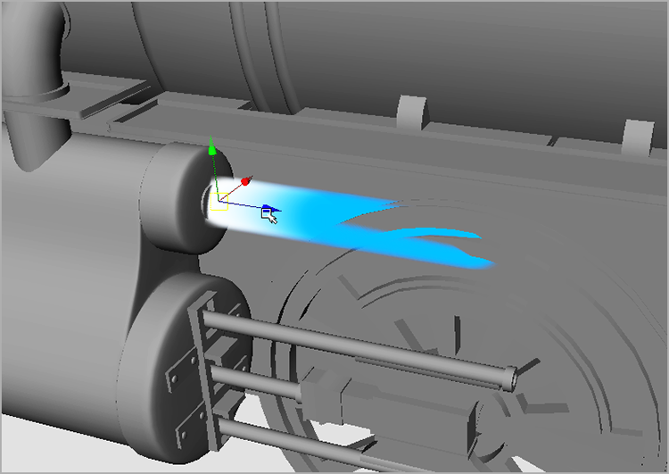
Figure 12-33: The emitter’s Spread attribute widens the spray of particles.

Figure 12-34: A range of offset between 0 and 0.3 units creates a more believable emission.

Setting nParticle Attributes
It’s always good to get the particles moving as closely to what you need as possible before you tend to their look. Now that you have the particles emitting properly from the steam pump, you’ll adjust the nParticle attributes. Start by setting a lifespan for them, and then add rendering attributes.
Figure 12-35: The initial radius settings for the steam nParticles

Figure 12-36: Open the Radius Scale ramp.

Figure 12-37: Decrease the radius of the nParticles using the Radius Scale ramp.

Figure 12-38: Adjust the Radius Scale ramp to grow the particles.

Figure 12-39: Select the meshes with which the nParticles will collide.
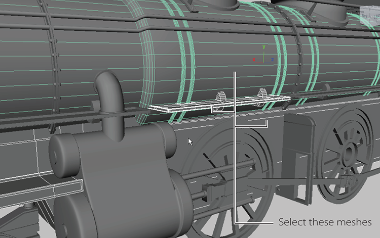
Figure 12-40: The particles now react very nicely against the side of the locomotive.

If you want to check your work, download the file locomotive_steam_v2.ma from the Locomotive project on the web page.
Setting Rendering Attributes
After you define the nParticle movement to your liking, you can create the proper look for the nParticles. This means setting and adjusting their rendering parameters.
Figure 12-41: Creating an Opacity ramp for the steam

Figure 12-42: The steam seems too short and small.

Figure 12-43: A better emission, but a bit too solid
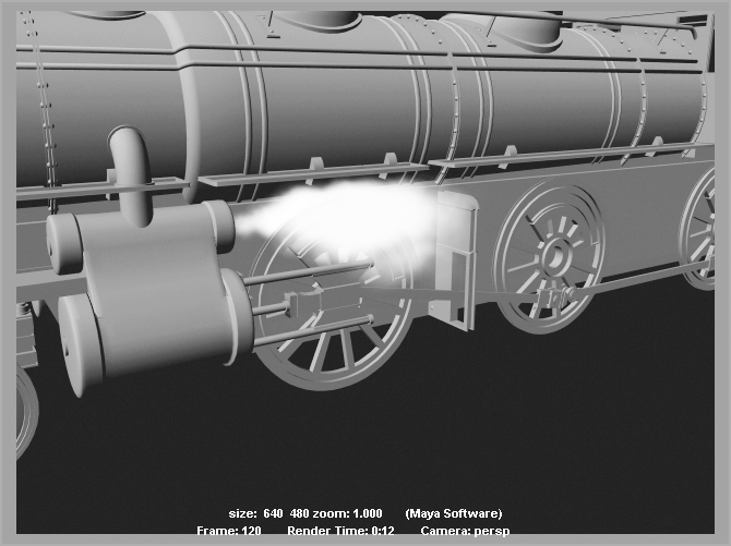
Figure 12-44: The shaders assigned to the cloud nParticle

Figure 12-45: The steam is less flat and solid.

Batch-render a 200-frame sequence of the scene at a lower resolution, such as 320×240, to see how the particles look as they animate. (Check the frames with FCheck. Refer to Chapter 11, “Autodesk Maya Rendering,” for more on FCheck.)
Download the file locomotive_steam_v3.ma from the Locomotive project on the web page to check your work.
Experiment with the steam by animating the Rate attribute of the emitter to make the steam pump out in time with the wheel arm. Also, try animating the Speed values and playing with different values in the Radius and Opacity ramps. The steam you’ll get in this tutorial looks pretty good, but it isn’t as lifelike as it could be. Particle animators are always learning new tricks and expanding their skills, and that comes from always trying new things and retrying the same effects with different methods.
When you feel comfortable with the steam exercise, try using the cloud nParticle to create steam for a mug of coffee. That steam moves much more slowly and is less defined than the blowing steam of the locomotive, and it should pose a new challenge. Also try your hand at creating a smoke trail for a rocket ship or a wafting stream of cigarette smoke, or even the billowing smoke coming from the engine’s chimney.
Cloud nParticles are the perfect particle type with which to begin. As you feel more comfortable animating with clouds, experiment with the other render types. The more you experiment with all the types of nParticles, the easier they will be to harness.
Introduction to Paint Effects
One of the tools in the effects arsenal of Maya is called Paint Effects. Using Paint Effects, you can create a field of grass rippling in the wind, a head of hair or feathers, or even a colorful aurora in the sky. Paint Effects is a rendering effect found in the Rendering menu. It has incredible dynamic properties that can make leaves rustle or trees sway in a storm. Paint Effects uses its own dynamics calculations to create natural motion. It’s one of the most powerful tools in Maya, with features that go far beyond the scope of this introductory book. Here you’ll learn how to create a Paint Effects scene and how to access all the preset brushes to create your own effects.
Paint Effects uses brushes to paint effects into your 3D scene. The brushes create strokes on a surface or in the Maya modeling views that produce tubes, which render out through the Maya Software renderer. These Paint Effects tubes have dynamic properties, which means they can move according to their own forces. Therefore, you can easily create a field of blowing grass.
Figure 12-46: The preset grass brushes in the Visor window
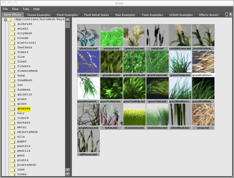
Figure 12-47: Click and drag two lines across the grid.

Figure 12-48: Add new strokes to add flowers to the grass.

Figure 12-49: Paint Effects can add realistic flowers and grass to any scene.

After you create a Paint Effects stroke, you can edit the look and movement of the effect through the Attribute Editor. You’ll notice, however, that there are a large number of attributes to edit with Paint Effects. The next section introduces the attributes that are most useful to the beginning Maya user.
Paint Effects Attributes
It’s best to create a single stroke of Paint Effects in a blank scene and experiment with adjusting the various attributes to see how they affect the strokes. Select the stroke, and open the Attribute Editor. Switch to the stroke’s tab to access the attributes. For example, for an African Lily Paint Effects stroke, the Attribute Editor tab is called africanLily1.
Each Paint Effects stroke produces tubes that render to create the desired effect. Each tube (you can think of a tube as a stalk) can grow to have branches, twigs, leaves, flowers, and buds. Each section of a tube has its own controls to give you the greatest flexibility in creating your effect. As you experiment with Paint Effects, you’ll begin to understand how each attribute contributes to the final look of the effect.
Here is a summary of some Paint Effects attributes:
In the Tubes section, you’ll find all the attributes to control the growth of the Paint Effects effect. In the Creation subsection, you can access the following:
In the Growth subsection, you can access controls for branches, twigs, leaves, flowers, and buds for the Paint Effects strokes. Each attribute in these sections controls the number, size, and shape of those elements. Although not all Paint Effects strokes create flowers, all strokes contain these headings.
The Behavior subsection contains the controls for the dynamic forces affecting the tubes in a Paint Effects stroke. Adjust these attributes if you want your flowers to blow more in the wind.
Paint Effects are rendered as a postprocess, which means they won’t render in reflections or refractions as is and they will not render in mental ray without conversion to polygons. They’re processed and rendered after every other object in the scene is rendered out in Maya Software rendering only.
To render Paint Effects in mental ray, you can convert Paint Effects to polygonal surfaces. They will then render in the scene along with any other objects so that they may take part in reflections and refractions. To convert a Paint Effects stroke to polygons, select the stroke and choose Modify ⇒ Convert ⇒ Paint Effects To Polygons. The polygon Paint Effects tubes can still be edited by most of the Paint Effects attributes mentioned so far; however, some, such as color, don’t affect the poly tubes. Instead, the color information is converted into a shader that is assigned to the polygons. It’s best to finalize your Paint Effects strokes before converting to polygons, to avoid any confusion.
Paint Effects is a strong Maya tool, and you can use it to create complex effects such as a field of blowing flowers. A large number of controls to create a variety of effects come with that complexity. Fortunately, Maya comes with a generous sampling of preset brushes. Experiment with a few brushes and their attributes to see what kinds of effects and strange plants you can create.
Toon Shading
Paint Effects has been developed into a toon-shading system to make your animations render more like traditional cartoons. Using Paint Effects, Maya renders outlines for the objects in your scene, and using a Toon shader, Maya renders the objects in the scene with a flat cartoon-color look. Next, you’ll take a quick look at how to apply toon shading to the wagon you textured in Chapter 7, “Autodesk Maya Shading and Texturing,” to make it render like a cartoon.
Figure 12-50: Select the main body of the wagon, without the wheels or the rails.
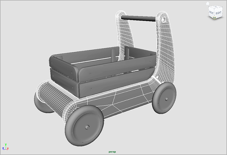
Figure 12-51: A Ramp shader is added to the scene and applied to the wagon’s body.

Figure 12-52: The wagon now has a toon-shaded body. The front side of the wagon is a darker red than the front because of the lighting in the scene.

Figure 12-53: The wagon has Toon shaders for the fill color applied.

Figure 12-54: The black outlines are applied, but they’re too thick.

Figure 12-55: The cartoon wagon

You can adjust the colors and the ramps of the fill shader to suit your tastes, and you can try the other Fill shader types, such as a three-tone shader to get a bit more detail in the coloring of the wagon. Adjust the toon outline thickness like you like, and have some fun playing with the toon outline’s attributes to see how they affect the toon rendering of the wagon. This should be a quick primer to get you into toon shading. The rest, as always, is up to you. With some playing and experimenting, you’ll be rendering some pretty nifty cartoon scenes in no time.
Getting Started with nCloth
nCloth, part of the nucleus dynamics in Autodesk Maya, is a simple yet very powerful way to create cloth simulations in your scene. From complex clothing on a moving character, to a simple flag, nCloth dynamics can create stunning movement, albeit with some serious setup. I will very briefly touch on the nCloth workflow here to give you a taste for it and familiarize you with the basics of getting started.
Making a Tablecloth
Switch to the nDynamics menu set. The nMesh menu is where you need to start to drape a simple tablecloth on a round table in the following steps:
Figure 12-56: Place a square plane above a flat cylinder.
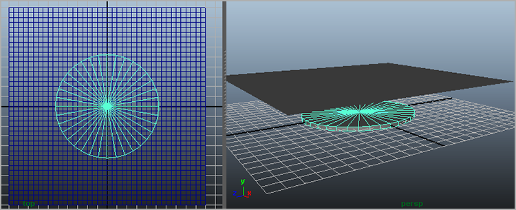
Figure 12-57: The cloth is working already!

Well, as easy as that was, there’s a lot more to it to achieve the specific effect you may need. But you’re on the road already. The first thing to understand is that the higher the resolution of the poly mesh, the better the look and movement of the cloth, at the cost of speed. At 40 subdivisions on the plane, the simulation runs pretty well, but you can see jagged areas of the tablecloth, so you would need to start with a much higher mesh for a smoother result.
Select the tablecloth, and open the Attribute Editor. There is a wide range of attributes to adjust for different cloth settings; however, you can choose from a number of built-in presets to make life easier. In the Attribute Editor, choose Presets*, as shown in Figure 12-58. Select Silk ⇒ Replace. As you can see, there are several Blend options in the submenu as well, allowing you to blend your current settings with the preset settings.
Figure 12-58: The built-in nCloth presets

In this case, you’ve chosen Replace to set the tablecloth object to simulate like Silk. It will be lighter and airier than before. Figure 12-59 (left) shows the tablecloth at frame 200 with the silk preset. Now, in the Attribute Editor, choose Preset ⇒ thickLeather ⇒ Replace for a heavier cloth simulation (Figure 12-59, right). Notice the playback for the heavy leather was slower as well.
Figure 12-59: The silk cloth simulation is lighter (left); leather simulation is heavier and runs slower.

As a beginner to Maya, it may be most helpful for you to go through the range of presets and see how the attributes for the nCloth changes. Here is a preliminary rundown of some of the nCloth attributes found under the Dynamic Properties heading in the Attribute Editor. Try changing some of these values to see how your tablecloth reacts, and you’ll gain a finer appreciation for the mechanics of nCloth.
Making a Flag
Now let’s make a very quick flag simulation to get familiar with nConstraints.
Figure 12-60: Create the mesh for the flag.

Figure 12-61: Select the vertices for the nConstraint.

Figure 12-62: The flag is tethered to an imaginary pole now.
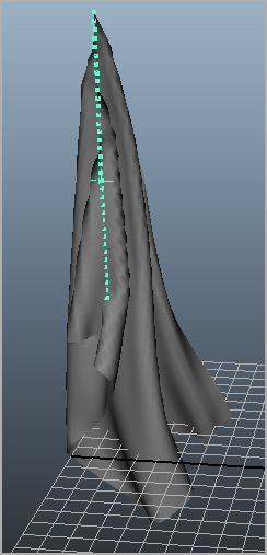
Figure 12-63: Wave the flag.

Adjust the Air Density, Wind Speed, Wind Direction, and Wind Noise attributes to adjust how the flag waves. You can use a similar workflow to create drapes blowing in an open window, for instance.
Caching an nCloth
Making a disk cache for a cloth simulation is important for better playback in your scene. Also, if you are rendering, it’s always a good idea to cache your simulation to avoid any issues. Caching an nCloth is very simple. Select the cloth object, such as the flag from the previous example, and in the Main Menu bar, choose nCache ⇒ Create New Cache ![]() . Figure 12-64 shows the options for the nCache. Here you can specify where the cache files are saved as well as the frame range for the cache. Once you create the cache, you will be able to scrub your playback back and forth.
. Figure 12-64 shows the options for the nCache. Here you can specify where the cache files are saved as well as the frame range for the cache. Once you create the cache, you will be able to scrub your playback back and forth.
Figure 12-64: Create nCache Options dialog box

In case you need to change your simulation, you will need to remove the cache first before changing nCloth or nucleus attributes. To do so, select the cloth object, and choose nCache ⇒ Delete Cache ![]() . In the option box, you can select whether you want to delete the cache files or just disconnect them from the nCloth object.
. In the option box, you can select whether you want to delete the cache files or just disconnect them from the nCloth object.
You can reattach an existing cache file by selecting the nCloth object and choosing nCache ⇒ Attach Existing Cache File. That existing cache must be from that object or one with the same topology.
Customizing Maya
One of the most endearing features of Maya is its almost infinite customizability. Everyone has different tastes, and everyone works in their own way. Simply put, for everything there is to do in Maya, you have several ways of doing it; there are at least a couple of ways to access the Maya tools, features, and functions as well.
This flexibility may be confusing at first, but you’ll discover that in the long run it’s very advantageous. The ability to customize enables the greatest flexibility in individual workflow.
It’s best to use Maya at its defaults as you first learn. However, when you feel comfortable enough with your progress, you can use this section to change some of the interface elements in Maya to better suit how you like to work.
User Preferences
All the customization features are found under Window ⇒ Settings/Preferences, which displays the window shown in Figure 12-65.
Figure 12-65: The Settings/Preferences menu

The Preferences window (see Figure 12-66) lets you make changes to the look of the program as well as to toolset defaults by selecting from the categories listed in the left pane of the window.
Figure 12-66: The Preferences window
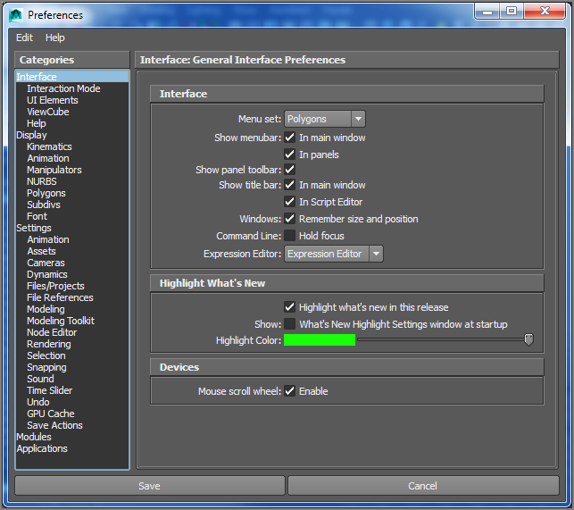
The Preferences window is separated into categories that define different aspects of the program. Interface and Display deal with options to change the look of the program. Interface affects the main user interface, whereas Display affects how objects are displayed in the workspace.
The Settings category lets you change the default values of several tools and their general operation. An essential aspect of this category is Working Units: these options set the working parameters of your scene (in particular, the Time setting).
By adjusting the Time setting, you tell Maya your frame rate of animation. If you’re working in film, you use a frame rate of 24 frames per second (fps). If you’re working in NTSC video (the standard video/television format in the Americas), you use the frame rate of 30fps.
The Applications category lets you specify which applications you want Maya to start automatically when a function is called. For example, while looking at the Attribute Editor for a texture image, you can click a single button to open that image in your favorite image editor, which you specify here.
Shelves
Under the Shelf Editor command (Window ⇒ Settings/Preferences ⇒ Shelf Editor) lurks a window that manages your shelves (see Figure 12-67). You can create or delete shelves or manage the items on the Shelf with this function. This is handy when you create your own workflow for a project. Simply click the Shelves tab to display the icons on that Shelf in the Shelf Editor window. Click in the Shelf Contents section to edit the icons and where they reside on that selected Shelf. Clicking the Command tab gives you access to the MEL command for that icon when it is single-clicked in the Shelf. Click the Double Click Command tab for the MEL command for the icon when it is double-clicked in the Shelf.
Figure 12-67: The Shelf Editor

You can also edit Shelf icons from within the UI without the Shelf Editor window. To add a menu command to the current Shelf, hold down Ctrl+Alt+Shift, and click the function or command directly from its menu. Items from the Tool Box, pull-down menus, or the Script Editor can be added to any Shelf.
- To add an item from the Tool Box, MMB+drag its icon from the Tool Box into the appropriate Shelf.
- To add an item from a menu to the current Shelf, hold down the Ctrl+Alt+Shift keys while selecting the item from the menu.
- To add an item (a MEL command) from the Script Editor, highlight the text of the MEL command in the Script Editor, and MMB+drag it onto the Shelf. A MEL icon will be created that will run the command when you click it.
- To remove an item from a Shelf, MMB+drag its icon to the Garbage Can icon at the end of the Shelf, or use Window ⇒ Settings/Preferences ⇒ Shelf Editor.
Hotkeys
Hotkeys are keyboard shortcuts that can access almost any Maya tool or command. You’ve already encountered a few in your exploration of the interface and in the solar system exercise in Chapter 2, “Jumping in Headfirst, with Both Feet.” What fun! You can create even more hotkeys, as well as reassign existing hotkeys, through the Hotkey Editor, shown in Figure 12-68 (Window ⇒ Settings/Preferences ⇒ Hotkey Editor).
Figure 12-68: The Hotkey Editor

Through this monolith of a window, you can set a key combination to be used as a shortcut to virtually any command in Maya. This is the last customization you want to touch. Because so many tools have hotkeys assigned by default, it’s important to get to know them first before you start changing things to suit how you work.
Every menu command is represented by menu categories on the left; the right side allows you to view the current hotkey or assign a new hotkey to the selected command. Ctrl and Alt key combinations may be used with any letter keys on the keyboard. Keep in mind that Maya is case sensitive, meaning that it differentiates between uppercase and lowercase letters. For example, one of my personal hotkeys is Ctrl+H to hide the selected object from view; Shift+Ctrl+H unhides it. (I’m sharing.)
The lower section of this window displays the MEL command that the menu command invokes. It also allows you to type in your own MEL commands, name them as new commands, categorize them with the other commands, and assign hotkeys to them.
Color Settings
You can set the colors for almost any part of the interface to your liking through the Colors window shown in Figure 12-69 (Window ⇒ Settings/Preferences ⇒ Color Settings).
Figure 12-69: Changing the interface colors is simple.

The window is separated into different aspects of the Maya interface by headings. The 3D Views heading lets you change the color of all the panels’ backgrounds. For example, color settings give you a chance to set the interface to complement your office’s décor as well as make certain items easier to read.
Customizing Maya is important. However—and this can’t be stressed enough—it’s important to get your bearings with default Maya settings before you venture out and change hotkeys and such. When you’re ready, this section of this chapter will still be here for your reference.
Summary
In this chapter, you learned how to create dynamic objects and create simulations. Beginning with rigid body dynamics, you created a set of pool balls that you animated in the simulation to knock into each other. Then, you learned how to bake that simulation into animation curves for fine-tuning. A quick fun exercise had you shooting the catapult, after which you learned about particle effects by creating a steam effect for the locomotive animation using nParticles. Next, you learned a little about the Maya Paint Effects tool and how you can easily use it to create various effects such as grass and flowers. Then you used toon shading on a wagon and finally glossed over some of the customization options available in the Maya UI. Then you learned how to create cloth effects using nCloth to make a tablecloth and a flag, and finally, you learned how to customize Maya to suit your own preferences.
To further your learning, try creating a scene on a grassy hillside with train tracks running through. Animate the locomotive, steam and all, driving through the scene and blowing the grass as it passes. You can also create a train whistle and a steam effect when the whistle blows, and you can create various other trails of smoke and steam as the locomotive drives through.
The best way to be exposed to Maya dynamics is simply to experiment once you’re familiar with the general workflow in Maya. You’ll find that the workflow in dynamics is more iterative than other Maya workflows, because you’re required to experiment frequently with different values to see how they affect the final simulation. With time, you’ll develop a strong intuition, and you’ll accomplish more complex simulations faster and with greater effect.
Where Do You Go from Here?
It’s so hard to say goodbye! But this is really a “hello” to learning more about animation and 3D!
Please explore other resources and tutorials to expand your working knowledge of Maya. Several websites contain numerous tips, tricks, and tutorials for all aspects of Maya, and my own resources and instructional videos and links are online at http://koosh3d.com/ and on Facebook at facebook.com/IntroMaya.
Of course, www.autodesk.com/maya has a wide range of learning tools. Be sure to check out the sidebar “Suggested Reading” in the absolutely fabulous Chapter 1, “Introduction to Computer Graphics and 3D.” Now that you’ve gained your all-important first exposure, you’ll be better equipped to forge ahead confidently.
The most important thing you should have learned from this book is that proficiency and competence with Maya come with practice, but even more so from your own artistic exploration. Treat this text and your experience with its information as a formal introduction to a new language and way of working for yourself; doing so is imperative. The rest of it—the gorgeous still frames and eloquent animations—come with furthering your study of your own art, working diligently to achieve your vision, and having fun along the way. Enjoy, and good luck.