10.4 ABC: Approximate Bayesian Computation
10.4.1 The ABC rejection algorithm
We sometimes find that we have a model with a likelihood which is mathematically difficult to deal with, and for such cases a technique called Approximate Bayesian Computation or ABC (sometimes referred to as likelihood-free computation) has been developed and has been quite widely employed, especially in genetics. There are several variants of this technique and we will illustrate each of them with the genetic linkage example we considered earlier in Sections 9.2 and 9.3.
Suppose we want to find the posterior distribution ![]() when we have observations
when we have observations ![]() coming from a distribution
coming from a distribution ![]() and a (proper) prior distribution
and a (proper) prior distribution ![]() for θ. Then if the observations come from a discrete distribution we can use the following algorithm to generate a sample of size k from the required posterior distribution.
for θ. Then if the observations come from a discrete distribution we can use the following algorithm to generate a sample of size k from the required posterior distribution.
10.4.1.1 ABC algorithm
This algorithm works because for any set A of possible values of θ we find (using the ‘tilde’ notation introduced in Chapter 1)

as required.
Although it works, this is an extremely inefficient algorithm. If, for example, we take six observations from a Poisson distribution such as the misprint data considered in Section 3.4

We could calculate the value of this for any conjugate prior
![]()
but for simplicity we consider the case where ![]() and S0=2, so that our prior is
and S0=2, so that our prior is ![]() . With the data we considered in that example, namely,
. With the data we considered in that example, namely, ![]() , the required probability becomes
, the required probability becomes

Clearly this technique is not practical without modification, even in the discrete case, and since continuous random variables attain any particular value with probability zero, it cannot be used at all in the continuous case.
We can make a slight improvement by use of sufficient statistics. So in the case of a sample of size 6 from ![]() we need consider only the sum
we need consider only the sum ![]() of the observations, which has a
of the observations, which has a ![]() distribution. With this in mind, we can replace step 3 of the algorithm by
distribution. With this in mind, we can replace step 3 of the algorithm by
3*. If ![]() , accept θ as an observation from
, accept θ as an observation from ![]() and otherwise reject
and otherwise reject ![]() .
.
By working with the sufficient statistic, the acceptance probability with the aforementioned data rises to

This is clearly not enough.
If there is a distance metric d available defining distances between values of the statistic T(x), we can define an ε-approximate posterior distribution ![]() as
as
![]()
where
![]()
10.4.1.2 ABC-REJ algorithm
With this modification, the method can be used with continuous random variables as well as with discrete ones. We observe that if ![]() this algorithm reduces to the previous one with the modification concerning sufficient statistics.
this algorithm reduces to the previous one with the modification concerning sufficient statistics.
Sometimes there is not a suitable sufficient statistic and we instead use a statistic ![]() which is in some sense close to being sufficient.
which is in some sense close to being sufficient.
10.4.2 The genetic linkage example
We shall now apply this method to the genetic linkage. Recall that we considered observations ![]() with cell probabilities
with cell probabilities
![]()
The values actually observed were x1=125, x2=18, x3=20, x4=34, and we are interested in the posterior distribution of ![]() . The likelihood is then
. The likelihood is then
![]()
and so ![]() is sufficient. We take a uniform U(0, 1) prior for
is sufficient. We take a uniform U(0, 1) prior for ![]() , use the distance measure
, use the distance measure
![]()
and fix a value for ε. The algorithm takes the form:
10.4.2.1 ABC-REJ algorithm for the genetic linkage example
![]()
A program in ![]() to do this is as follows:
to do this is as follows:
N <- 100000
etastar <- c(125,18+20,34)
n <- sum(etastar)
eps <- 3
d <- rep(NA,N)
trial <- rep(NA,N)
for (j in 1:N) {
 etatrial <- runif(1)
 inds <- sample(3,n,replace=T,
      p=c(0.5+etatrial/4,(1-etatrial)/2,etatrial/4))
 samp <- c(sum(inds==1),sum(inds==2),sum(inds==3))
 d <- sqrt(sum((etastar-samp)^2))
 if (d <= eps) trial[j] <- etatrial
}
eta <- trial[!is.na(trial)]
k <- length(eta)
m <- mean(eta)
s <- sd(eta)
cat("k",k,"m",m,"s",s,"
")
A run of this program produced a sample of values of ![]() of size k=1040, mean m=0.625 and s.d. s=0.0511. For comparison, we recall that we found a value for
of size k=1040, mean m=0.625 and s.d. s=0.0511. For comparison, we recall that we found a value for ![]() of 0.630 from the EM algorithm in Section 9.2, and a distribution with a posterior mode of 0.627 by data augmentation in Section 9.3.
of 0.630 from the EM algorithm in Section 9.2, and a distribution with a posterior mode of 0.627 by data augmentation in Section 9.3.
An ad hoc rule sometimes quoted is that ε should be chosen such that approximately 1% of trials of ![]() should be accepted, and the choice of 3 as a value for ε was made for this reason.
should be accepted, and the choice of 3 as a value for ε was made for this reason.
10.4.3 The ABC Markov Chain Monte Carlo algorithm
We can incorporate the idea of the Metropolis–Hastings algorithm introduced in Section 9.6 into approximate Bayesian computation. In the aforementioned algorithm ![]() is a suitable proposal density (a transition probability density for a Markov chain) and
is a suitable proposal density (a transition probability density for a Markov chain) and
![]()
where
![]()
the statistic ![]() being in some sense close to being sufficient.
being in some sense close to being sufficient.
10.4.3.1 ABC-MCMC algorithm
In the genetic linkage example [using the sufficient statistic ![]() as our
as our ![]() )] a convenient choice is a uniform prior U(0, 1) and a normal proposal density
)] a convenient choice is a uniform prior U(0, 1) and a normal proposal density
![]()
because, as is easily checked, ![]() then reduces to unity, and so
then reduces to unity, and so
![]()
The algorithm thus becomes:
10.4.3.2 ABC-MCMC algorithm for the genetic linkage example
A program in ![]() to do this is as follows:
to do this is as follows:
N <- 100000
epsilon <- 3
sdev <- 0.05
k <- 0
etaset <- 0.5
xstar <- c(125,18+20,34)
n <- sum(xstar)
eta <- rep(NA,N)
for (j in 1:N) {
 etatrial = rnorm(1,etaset,sdev)
 if ((0<etatrial)&(etatrial<1)) {
  inds <- sample(3,n,replace=T,
         prob=c((0.5+etatrial/4),((1-etatrial)/2),
         (etatrial/4)))
  x <- c(sum(inds==1),sum(inds==2),sum(inds==3))
  dist <- sqrt(sum((xstar-x)^2))
  if (dist <= epsilon) {
   etaset <- etatrial
   k <- k + 1
  }
 }
eta[j] <- etaset
}
m <- mean(eta)
s <- sd(eta)
cat("k",k,"m",m,"s",s,"
")}
A run of this program produced a sample of values of ![]() of size k=4627, mean m=0.624 and s.d. s=0.0499. Note the number of acceptances is some four and a half times as great as with the ABC-REJ algorithm.
of size k=4627, mean m=0.624 and s.d. s=0.0499. Note the number of acceptances is some four and a half times as great as with the ABC-REJ algorithm.
A problem which can occur with this algorithm is pointed out by Sisson et al. (2007). In their words, ‘if the ABC-MCMC sampler enters an area of relatively low probability with a poor proposal mechanism, the efficiency of the algorithm is strongly reduced because it then becomes difficult to move anywhere with a reasonable chance of acceptance, and so the sampler “sticks” in that part of the state space for long periods of time.’
10.4.4 The ABC Sequential Monte Carlo algorithm
In the ABC-SMC algorithm we try to improve on simple rejection sampling by adopting a sequential Monte Carlo based simulation approach. Here, a collection of values ![]() from the parameter space (termed particles) is propagated from an initial prior distribution through a sequence of intermediary distributions, until it ultimately represents the target distribution. The method can be thought of as a type of importance sampling (cf. Section 10.1).
from the parameter space (termed particles) is propagated from an initial prior distribution through a sequence of intermediary distributions, until it ultimately represents the target distribution. The method can be thought of as a type of importance sampling (cf. Section 10.1).
We begin by taking ![]() from an initial distribution
from an initial distribution ![]() (which may or may not be the prior distribution p). We then seek a target distribution
(which may or may not be the prior distribution p). We then seek a target distribution ![]() which represents the posterior of θ conditional on
which represents the posterior of θ conditional on ![]() for observed data
for observed data ![]() . The standard importance sampling procedure would then indicate how well each particle
. The standard importance sampling procedure would then indicate how well each particle ![]() adheres to
adheres to ![]() by specifying the importance weight
by specifying the importance weight ![]() it should receive in the full population of N particles. The effectiveness of such a procedure is sensitive to the choice of
it should receive in the full population of N particles. The effectiveness of such a procedure is sensitive to the choice of ![]() and it can be highly inefficient if
and it can be highly inefficient if ![]() is diffuse relative to fT.
is diffuse relative to fT.
The idea behind sequential sampling methods is to avoid the potential disparity between ![]() and fT by specifying a sequence of intermediary distributions
and fT by specifying a sequence of intermediary distributions ![]() such that they evolve gradually from the initial distribution towards the target distribution. In the ABC setting, we may naturally define the sequence of distributions
such that they evolve gradually from the initial distribution towards the target distribution. In the ABC setting, we may naturally define the sequence of distributions ![]() as
as
![]()
where ![]() is a strictly decreasing sequence of tolerances.
is a strictly decreasing sequence of tolerances.
The degree of sample degeneracy in a population is measured by the effective sample size ESS which represents the equivalent number of random samples needed to obtain an estimate such that its Monte Carlo variation is equal to that of the N weighted particles and it may be estimated as ![]() , which is between 1 and N. It is usual to set a re-sampling threshold E, which is often taken as N/2.
, which is between 1 and N. It is usual to set a re-sampling threshold E, which is often taken as N/2.
A difficulty with this approach is that, while some action occurs (e.g. a realization or move proposal is accepted) each time a non-zero likelihood is encountered, there is a large probability that the likelihood, and therefore the particle weight will be zero. Fortunately, the idea of partial rejection control leads to the modified notion of the ABC-PRC algorithm.
This process can be described in the following algorithm which assumes that data ![]() is available and is taken from the 2009 corrections to Sisson et al. (2007):
is available and is taken from the 2009 corrections to Sisson et al. (2007):
10.4.4.1 ABC-PRC algorithm
![]()
Note that as ![]() is the prior density, when t=1 step 2(b) gives the same weights as in importance sampling in Section 10.1, while the weights when t> 1 come from an obvious updating process.
is the prior density, when t=1 step 2(b) gives the same weights as in importance sampling in Section 10.1, while the weights when t> 1 come from an obvious updating process.
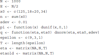
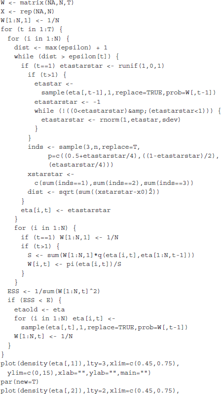
An ![]() program to carry this out for the genetic linkage example, using the normal random walk (restricted, so that
program to carry this out for the genetic linkage example, using the normal random walk (restricted, so that ![]() is always between 0 and 1) as the Markov transition density, is as follows:
is always between 0 and 1) as the Markov transition density, is as follows:


Estimated density functions of ![]() based on
based on ![]() ,
, ![]() and
and ![]() are shown in Figure 10.4.
are shown in Figure 10.4.
Figure 10.4 The ABC-PRC algorithm for the genetic linkage example.

10.4.5 The ABC local linear regression algorithm
Another variant of ABC which has been proposed uses local linear regression. We shall illustrate the technique in the case where there is a single unknown parameter θ. We define the Epanechnikov kernel as the function
![]()
so that ![]() and
and ![]() . We then use this function to give most weights to those simulations which result in the smallest values of
. We then use this function to give most weights to those simulations which result in the smallest values of ![]() . Thus, we could estimate the mean value of θ by
. Thus, we could estimate the mean value of θ by
![]()
But actually we can go further than this. We can seek values of α and ![]() which minimize
which minimize
![]()
If instead of using the Epanechnikov kernel, we had taken ![]() for all t this would result in ordinary linear regression as we considered in Section 6.3, but instead we are giving more weight to observations for which
for all t this would result in ordinary linear regression as we considered in Section 6.3, but instead we are giving more weight to observations for which ![]() is small. Straightforward differentiation shows that
is small. Straightforward differentiation shows that

By setting ![]() we see that the minimum occurs when
we see that the minimum occurs when ![]() and
and ![]() , where
, where

and these equations are easily solved, albeit not quite as simply as in Section 6.3 since ![]() does not drop out of the first equation.
does not drop out of the first equation.
The natural way of solving such equations is by matrix algebra and with matrix techniques it is almost as easy to deal with cases where the statistic ![]() is multidimensional. For details see Beaumont et al. (2002).
is multidimensional. For details see Beaumont et al. (2002).
10.4.6 Other variants of ABC
Various other variants of the ABC technique have been considered, such as non-linear regression models, in particular fast-forward neural network regression models. For details, see Blum and François (2010).
It has also been applied to model selection (see Toni and Stumpf, 2010).
A forthcoming paper likely to be of interest in connection with ABC is Fearnhead and Prangle (2012) and a useful survey is Sisson and Fan (2011).
