
9.5 Rejection sampling
9.5.1 Description
An important method which does not make use of Markov chain methods but which helps to introduce the Metropolis–Hastings algorithm is rejection sampling or acceptance-rejection sampling. This is a method for use in connection with a density ![]() in the case where the normalizing constant K is quite possibly unknown, which, as remarked at the beginning of this chapter, is a typical situation occurring in connection with posterior distributions in Bayesian statistics. To use this method, we need to assume that there is a candidate density
in the case where the normalizing constant K is quite possibly unknown, which, as remarked at the beginning of this chapter, is a typical situation occurring in connection with posterior distributions in Bayesian statistics. To use this method, we need to assume that there is a candidate density ![]() from which we can simulate samples and a constant c such that
from which we can simulate samples and a constant c such that ![]() . Then, to obtain a random variable
. Then, to obtain a random variable ![]() with density
with density ![]() we proceed as follows:
we proceed as follows:
In the discrete case we can argue as follows. In N trials we get the value θ on ![]() occasions, of which we retain it
occasions, of which we retain it ![]() times, which is proportional to
times, which is proportional to ![]() . Similar considerations apply in the continuous case; a formal proof can be found in Ripley (1987, Section 3.2) or Gamerman and Lopes (2011, Section 5.1).
. Similar considerations apply in the continuous case; a formal proof can be found in Ripley (1987, Section 3.2) or Gamerman and Lopes (2011, Section 5.1).
9.5.2 Example
As a simple example, we can use this method to generate values X from a beta distribution with density f(x)/K, where ![]() in the case where
in the case where ![]() and
and ![]() (in fact, we know that in this case
(in fact, we know that in this case ![]() and
and ![]() ). We simply note that the density has a maximum at
). We simply note that the density has a maximum at ![]() (see Appendix A), so that we can take
(see Appendix A), so that we can take ![]() and h(x)=1, that is,
and h(x)=1, that is, ![]() as well as
as well as ![]() .
.
9.5.3 Rejection sampling for log-concave distributions
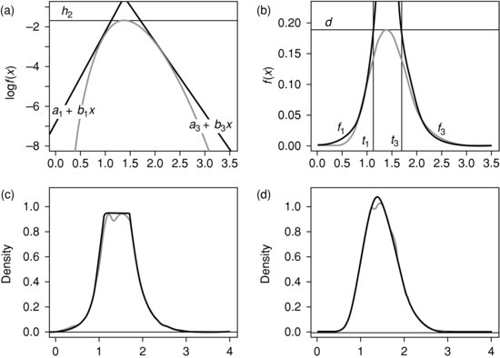
It is often found that inference problems simplify when a distribution is log-concave, that is when the logarithm of the density function is concave (see Walther, 2009). In such a case, we can fit a piecewise linear curve over the density as depicted in Figure 9.4a. In that particular case, there are three pieces to the curve, but in general there could be more. Exponentiating, we find an upper bound for the density itself which consists of curves of the form exp(a+bx), as depicted in Figure 9.4b. As these curves are easily integrated, the proportions of the area under the upper bound which fall under each of the curves are easily calculated. We can then generate a random variable with a density proportional to the upper bound in two stages. We first choose a constituent curve exp(a+bx) between x=t and ![]() with a probability proportional to
with a probability proportional to
Figure 9.4 Rejection sampling: (a) log density, (b) un-normalized density, (c) empirical density before rejection and (d) empirical density of v.
![]()
After this, a point between t and ![]() is chosen as a random variable with a density proportional to exp(a+bx).
is chosen as a random variable with a density proportional to exp(a+bx).
For the latter step, we note that such a random variable has distribution function
![]()
The inverse function of this is easily shown to be
![]()
If then V is uniformly distributed over [0, 1] and we write X=F–1(V), it follows that
![]()
so that X has the distribution function f(x).
Figure 9.4c show that simulation using this method produces an empirical distribution which fits closely to the upper envelope of curves we have chosen. We can now use the method of rejection sampling as described earlier to find a sample from the original log-concave density. The empirical distribution thus produced is seen to fit closely to this density in Figure 9.4d.
The choice of the upper envelope can be made to evolve as the sampling proceeds; for details, see Gilks and Wild (1992).
9.5.4 A practical example
In Subsection 9.4.2 headed ‘An example with observed data’ which concerned pump failures, we assumed that the parameter ν was known to be equal to 1.4. It would clearly be better to treat ν as a parameter to be estimated in the same way that we estimated S. Now
![]()
since the distribution of ![]() given
given ![]() does not depend on ν or S0. Consequently
does not depend on ν or S0. Consequently
![]()
Unfortunately, the latter expression is not proportional to any standard family for any choice of hyperprior ![]() . If, however,
. If, however,
![]()
has the form of an exponential distribution of mean μ, we find that

so that
![]()
The logarithm of this density is convex. A proof of this follows, but the result can be taken for granted. We observe that the first derivative of the density is
![]()
where
![]()
(cf. Appendix A.7), while the second derivative is
![]()
where ![]() is the so-called trigamma function.
Since the trigamma function satisfies
is the so-called trigamma function.
Since the trigamma function satisfies
![]()
(see Whittaker and Watson, 1927, Section 12.16), it is clear that this second derivative is negative for all z> 0, from which convexity follows.
We now find a piecewise linear function which is an upper bound of the density in the manner described earlier. In this case, it suffices to approximate by a three-piece function, as illustrated in Figure 9.4a. This function is constructed by taking a horizontal line tangent at the zero n2 of the derivative of the log-density, where this achieves its maximum h2 and then taking tangents at two nearby points n1 and n3. The joins between the lines occur at the points t1 and t3 where these three curves intersect. Exponentiating, this gives an upper bound for the density itself, consisting of a number of functions of the form exp(a+bx) (the central one being a constant), as illustrated in Figure 9.4b.
In this case, the procedure is very efficient and some 87–88% of candidate points are accepted. The easiest way to understand the details of this procedure is to consider the ![]() program:
program:
windows(record=T)
par(mfrow=c(2,2))
N < - 5000
mu < - 1
S < - 1.850
theta < - c(0.0626,0.1181,0.0937,0.1176,0.6115,
0.6130,0.8664,0.8661,1.4958,1.9416)
k < - length(theta)
logf < - function(nu) {
k*(nu/2)*log(S)-k*(nu/2)*log(2)-k*log(gamma(nu/2))+
(nu/2-1)*sum(log(theta))-nu/mu
)
dlogf < - function(nu) {
(k/2)*log(S)-(k/2)*log(2)-0.5*k*digamma(nu/2)+
0.5*sum(log(theta))-1/mu
}
scale < - 3/2
f < - function(nu) exp(logf(nu))
n2 < - uniroot(dlogf,lower=0.01,upper=100)$root
h2 < - logf(n2)
n1 < - n2/scale
h1 < - logf(n1)
b1 < - dlogf(n1)
a1 < - h1-n1*b1
n3 < - n2*scale
h3 < - logf(n3)
b3 < - dlogf(n3)
a3 < - h3-n3*b3
d < - exp(h2)
# First plot; Log density
curve(logf,0.01,3.5,ylim=c(-8,-1),xlab=“a. Log density”)
abline(h=h2)
abline(a1,b1)
abline(a3,b3)
text(0.25,h2+0.3,expression(italic(h)[2])))
text(0.3,-6,
expression(italic(a)[1]+italic(b)[1]*italic(x)))
text(3.25,-7,)
expression(italic(a)[3]+italic(b)[3]*italic(x)))
# End of first plot
f1 < - function(x) exp(a1+b1*x)
f3 < - function(x) exp(a3+b3*x)
t1 < - (h2-a1)/b1
t3 < - (h2-a3)/b3
# Second plot; Un-normalized density
curve(f,0.01,3.5,ylim=c(0,0.225),
xlab=“b. Un-normalized Density”)
abline(h=d)
par(new=T)
curve(f1,0.01,3.5,ylim=c(0,0.225),ylab="",xlab="")
par(new=T)
curve(f3,0.01,3.5,ylim=c(0,0.225),ylab="",xlab="")
abline(v=t1)
abline(v=t3)
text(t1-0.1,0.005,expression(italic(t)[1]))
text(t3-0.1,0.005,expression(italic(t)[3]))
text(0.25,0.2,expression(italic(d)))
text(0.5,0.025,expression(italic(f)[1]))
text(2.5,0.025,expression(italic(f)[3]))
# End of second plot
q1 < - exp(a1)*(exp(b1*t1)-1)/b1
q2 < - exp(h2)*(t3-t1)
q3 < - -exp(a3+b3*t3)/b3
const < - q1 + q2 + q3
p < - c(q1,q2,q3)/const
cat(“p =”,p,“
”)
case < - sample(1:3,N,replace=T,prob=p)
v < - runif(N)
w < - (case==1)*(1/b1)*log(q1*b1*exp(-a1)*v+1)+
(case==2)*(t1+v*(t3-t1))+
)*(1/b3)*(log(q3*b3*exp(-a3)*v+exp(b3*t3)))
dq < - d/const
f1q < - function(x) f1(x)/const
f3q < - function(x) f3(x)/const
h < - function(x) {
dq +
(x<t1)*(f1q(x)-dq) +
(x>t3)*(f3q(x)-dq)
}
# Third plot; Empirical density
plot(density(w),xlim=c(0.01,4),ylim=c(0,1.1),
xlab=“c. Empirical density before rejection”,
main="")
par(new=T)
curve(h,0.01,4,ylim=c(0,1.1),ylab="",xlab="")
# End of third plot
u < - runif(N)
nu < - w
nu[u>f(nu)/(const*h(nu))] < - NA
nu < - nu[!is.na(nu)]
cat(“Acceptances”,100*length(nu)/length(w),“
”)
int < - integrate(f,0.001,100)$value
fnorm < - function(x) f(x)/int
# Fourth plot
plot(density(nu),xlim=c(0.01,4),ylim=c(0,1.1),
xlab=bquote(paste(“d. Empirical density of ”,nu)),
main="")
par(new=T)
curve(fnorm,0.01,4,ylim=c(0,1.1),ylab="",xlab="")
# End of fourth plot}
It is possible to combine this procedure with the method used earlier to estimate the ![]() and S0, and an
and S0, and an ![]() program to do this can be found on the web. We shall not discuss this matter further here since it is in this case considerably simpler to use WinBUGS as noted in Section 9.7.
program to do this can be found on the web. We shall not discuss this matter further here since it is in this case considerably simpler to use WinBUGS as noted in Section 9.7.