8.6 The general linear model revisited

8.6.1 An informative prior for the general linear model

This section follows on from Section 6.7 on ‘The general linear model’ and like that section presumes a knowledge of matrix theory.

We suppose as in that section that

(where is r-dimensional, so is ), but this time we take a non-trivial prior for , namely

(where is s-dimensional, so is ). If the hyperparameters are known, we may as well take r=s and , and in practice dispense with , but although for the moment we assume that is known, in due course we shall let have a distribution, and it will then be useful to allow other values for .

Assuming that , and are known, the log of the posterior density is (up to an additive constant)

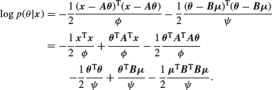
Differentiating with respect to the components of we get a set of equations which can be written as one vector equation

Equating this to zero to find the mode of the posterior distribution, which by symmetry equals its mean, we get

so that

In particular, if is taken as zero, so that the vector of prior means vanishes, then this takes the form

The usual least squares estimators reappear if .

8.6.2 Ridge regression

This result is related to a technique which has become popular in recent years among classical statisticians which is known as ridge regression. This was originally developed by Hoerl and Kennard (1970), and a good account of it can be found in the article entitled ‘Ridge Regression’ in Kotz et al. (2006); alternatively, see Weisberg (2005, Section 11.2). Some further remarks about the connection between ridge regression and Bayesian analysis can be found in Rubin (1988).

What they pointed out was that the appropriate (least squares) point estimator for was

From a classical standpoint, it then matters to find the variance–covariance matrix of this estimator in repeated sampling, which is easily shown to be

(since ), so that the sum of the variances of the regression coefficients is

(the trace of a matrix being defined as the sum of the elements down its main diagonal) and the mean square error in estimating θ is

However, there can be considerable problems in carrying out this analysis. It has been found that the least squares estimates are sometimes inflated in magnitude, sometimes have the wrong sign, and are sometimes unstable in that radical changes to their values can result from small changes or additions to the data. Evidently if is large, so is the mean-square error, which we can summarize by saying that the poorer the conditioning of the matrix, the worse the deficiencies referred to above are likely to be. The suggestion of Hoerl and Kennard was to add small positive quantities to the main diagonal, that is to replace by where k> 0, so obtaining the estimator

which we derived earlier from a Bayesian standpoint. On the other hand, Hoerl and Kennard have some rather ad hoc mechanisms for deciding on a suitable value for k.

8.6.3 A further stage to the general linear model

We now explore a genuinely hierarchical model. We supposed that , or slightly more generally that

(see the description of the multivariate normal distribution in Appendix A). Further a priori , or slightly more generally

At the next stage, we can suppose that our knowledge of is vague, so that . We can then find the marginal density of as

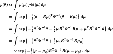
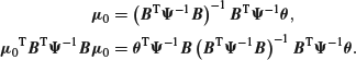
on completing the square by taking such that

that is

Since the second exponential is proportional to a normal density, it integrates to a constant and we can deduce that

that is , where

We can then find the posterior distribution of given as

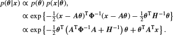
Again completing the square, it is easily seen that this posterior distribution is where

8.6.4 The one way model

If we take the formulation of the general linear model much as we discussed it in Section 6.7, so that

we note that . We assume that the xi are independent and have variance so that reduces to and hence The situation where we assume that the are independently fits into this situation if take (an r-dimensional column vector of 1s, so that while is an matrix with 1s everywhere) and have just one scalar hyperparameter μ of which we have vague prior knowledge. Then reduces to and to giving

and so has diagonal elements ai+b and all off-diagonal elements equal to b, where

These are of course the same values we found in Section 8.5 earlier. It is, of course, also be possible to deduce the form of the posterior means found there from the approach used here.

8.6.5 Posterior variances of the estimators

Writing

and (remember that b< 0) it is easily seen that

and hence

using the Sherman–Morrison formula for the inverse of with . [This result is easily established; in case of difficulty, refer to Miller (1987, Section 3) or Horn and Johnson (1991, Section 0.7.4).]  Consequently the posterior variance of is

Now substituting and ,we see that

from which it follows that

We thus confirm that the incorporation of prior information has resulted in a reduction of the variance.