1. Show that the prior

suggested in connection with the example on risk of tumour in a group of rats is equivalent to a density uniform in .

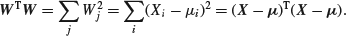
2. Observations x1, x2, … , xn are independently distributed given parameters , , … , according to the Poisson distribution . The prior distribution for is constructed hierarchically. First, the s are assumed to be independently identically distributed given a hyperparameter according to the exponential distribution for and then is given the improper uniform prior for . Provided that , prove that the posterior distribution of has the beta form

Thereby show that the posterior means of the are shrunk by a factor relative to the usual classical procedure which estimates each of the by xi.
What happens if ?

3. Carry out the Bayesian analysis for known overall mean developed in Section 8.2 mentioned earlier (a) with the loss function replaced by a weighted mean

and (b) with it replaced by

4. Compare the effect of the Efron–Morris estimator on the baseball data in Section 8.3 with the effect of a James–Stein estimator which shrinks the values of towards or equivalently shrinks the values of Xi towards .

5. The Helmert transformation is defined by the matrix

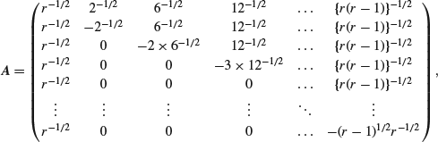
so that the element aij in row i, column j is

It is also useful to write for the (column) vector which consists of the jth column of the matrix . Show that if the variates Xi are independently , then the variates are independently normally distributed with unit variance and such that for j> 1 and

By taking for i> j, aij=0 for i< j and ajj such that , extend this result to the general case and show that . Deduce that the distribution of a non-central chi-squared variate depends only of r and .

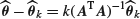
6. Show that where

(Lehmann 1983, Section 4.6, Theorem 6.2).

7. Writing

for the least-squares and ridge regression estimators for regression coefficients , show that

and that the bias of is

while its variance–covariance matrix is

Deduce expressions for the sum of the squares of the biases and for the sum of the variances of the regression coefficients, and hence show that the mean square error is

Assuming that is continuous and monotonic decreasing with and that is continuous and monotonic increasing with 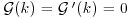, deduce that there always exists a k such that MSEk< MSE0 (Theobald, 1974).

8. Show that the matrix in Section 8.6 satisfies and that if is square and non-singular then vanishes.

9. Consider the following particular case of the two way layout. Suppose that eight plots are harvested on four of which one variety has been sown, while a different variety has been sown on the other four. Of the four plots with each variety, two different fertilizers have been used on two each. The yield will be normally distributed with a mean θ dependent on the fertiliser and the variety and with variance . It is supposed a priori that the mean for plots yields sown with the two different varieties are independently normally distributed with mean α and variance , while the effect of the two different fertilizers will add an amount which is independently normally distributed with mean β and variance . This fits into the situation described in Section 8.6 with being times an identity matrix and

Find the matrix needed to find the posterior of θ.

10. Generalize the theory developed in Section 8.6 to deal with the case where and and knowledge of is vague to deal with the case where (Lindley and Smith, 1972).

11. Find the elements of the variance–covariance matrix for the one way model in the case where ni=n for all i.