3

MODERN CONTROL-SYSTEM DESIGN USING STATE-SPACE, POLE PLACEMENT, ACKERMANN'S FORMULA, ESTIMATION, ROBUST CONTROL, AND H^∞ TECHNIQUES

3.1. INTRODUCTION

State-space analysis was introduced in Chapter 1, and has been used in parallel with the classical frequency-domain analyses techniques presented in Chapter 2. The state-space approach is applicable to a wider class of problems such as multiple-input/multiple-output (MIMO) control systems. Chapter 2 applied the frequency-domain approaches such as the Bode diagram, and the root locus to linear control-system design.

In the design of a control system, the question arises as to where to place the closed-loop roots. In Section 2.9 which presented the root-locus method, we could specify where to place the dominant-pair of complex-conjugate roots in order to obtain a desired transient response. However, we could not do so with great certainty because we were never sure what effect the higher-order poles would have on the second-order approximation.

The control-system design engineer desires to have design methods available which would enable the design to proceed by specifying all of the closed-loop poles of higher-order control systems. Unfortunately, the frequency-domain design methods presented in Chapter 2 do not permit the control-system engineer to specify all poles in control systems which are higher than two because they do not provide a sufficient number of unknowns for solving uniquely for the specified closed-loop poles. This problem is overcome using state-space methods which provide additional adjustable parameters, and methods for determining these parameters.

This chapter presents a modern control-system design method using state-space techniques known as pole placement or pole assignment. This design technique is similar to what we did in Section 2.9 where we placed two dominant complex-conjugate poles of the closed-loop transfer function in desired locations in order to obtain desirable transient responses. However, in this chapter, we will show how pole placement allows the control-system engineer to place all of the poles of the closed-loop transfer function in desirable locations. Ackermann's formula is also presented for designs using pole placement for application in those control systems that require feedback from state variables which are not phase variables (where each subsequent state variable is defined as the derivative of the previous state variable). A practical problem arises with the pole placement method involving cost and the availability of determining (measuring) all of the system variables needed for obtaining a solution. In many practical control systems, all of the system state variables may not be available due to cost considerations, environmental considerations (e.g., nuclear power plant control systems), and the availability of transducers to measure certain states. For these cases, it is necessary for the control-system engineer to estimate the state variables that cannot be measured from the state variables that can be measured. Therefore, in addition to pole placement, this chapter also presents the very important subjects of controllability, observability, and estimation.

This chapter on modern control-system design also presents the design of robust control systems. Robust control systems are concerned with determining a stabilizing controller that achieves feedback performance in terms of stability and accuracy requirements, but the controller must achieve performance that is robust (insensitive) to plant uncertainty, parameter variation, and external disturbances. The design of two-degrees-of-freedom compensation control systems exhibiting desirable robustness to plant uncertainty, parameter variation, and external disturbances is presented.

This chapter concludes with an introduction to H^∞ control concepts which is a new technique that emerged in the 1980s that combines both the frequency- and time-domain approaches to provide a unified design approach. The H^∞ approach has dominated the trend of control-system development in the 1980s and 1990s. The H^∞ control-system design approach expands on the concept of robustness presented in this chapter, sensitivity (presented in Chapter 1), together with the frequency and state-variable domain techniques presented in this book. The H^∞ approach is applied to determine the optimum sensitivity for control systems.

3.2. POLE-PLACEMENT DESIGN USING LINEAR-STATE-VARIABLE FEEDBACK

Having presented methods for designing linear control systems using classical techniques, let us now look at the problem of specifying pole placement from the viewpoint of state-variable feedback [1]. In order to do this, let us first look at the basic feedback problem illustrated in Figure 3.1. This figure illustrates the concept of feeding back the states of the process in addition to that of the output. Because a linear process can be characterized by the phase-variable canonical equations

Figure 3.1 General feedback system problem illustrating feedback of the output state and the states of the process.

let us consider the configuration of Figure 3.2. It is important to observe from this figure that the control signal is generated from a knowledge of the reference input r(t) and the state variables x(t). Note that r(t), u(t), and c(t) represent scalars.

In general, the control input u can be represented as

Rather than considering the controller in such a broad sense, let us consider the specific condition of linear state-variable feedback where the controller weights the sum of the state variables in a linear manner. In addition, it is assumed that the controller provides a linear gain K which multiplies the difference between the reference input and the linear weighted sum of state variables fed back. Therefore, u(t) can be represented as

where h_i is defined as the ith feedback coefficient. In matrix form, u(t) can be represented as

where

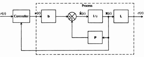
Figure 3.2 General feedback system with state-variable feedback.

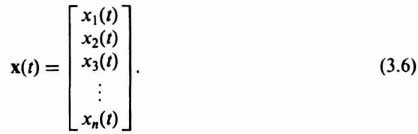
Figure 3.3 presents a matrix representation of the concept of linear-state-variable feedback, and Figure 3.4 is an example of a physical representation of a typical system as implied by Figure 3.3. In the following discussion, it is assumed that all state variables are directly available for measurement and control. In practice, this is not always possible, and techniques for modifying and extending the design procedure presented, to the case where all the state variables are not available, are also discussed in Sections 3.6 and 3.7.

How does linear feedback of the state variables affect the behavior of the process given by Eqs. (3.1) and (3.2)? This can easily be determined by substituting Eq. (3.4) into Eq. (3.1):

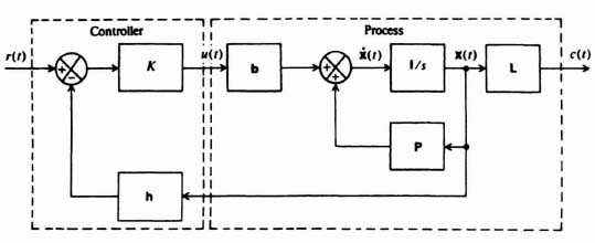
Figure 3.3 Linear-state-variable feedback representation.

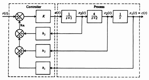
Figure 3.4 Example of pole placement design using linear-state-variable feedback.

Simplifying Eq. (3.7), and incorporating Eq. (3.2), we obtain the closed-loop equation

where

is the closed-loop-system matrix. Comparing Eq. (3.1) and (3.2) with (3.8) and (3.9), we observe that they are identical except that the P matrix has been replaced by P_h and u(t) becomes Kr(t).

How can we relate the closed-loop-system matrix P_h to the closed-loop transfer function, C(s)/R(s)? This can be accomplished by taking the Laplace transform of Eqs. (3.8) and (3.9). Because the results will be used to find a transfer function, all initial conditions are assumed to be zero:

Solving for X(s) from Eq. (3.11), we get

The inverse matrix [sI – P_h]⁻¹ is defined as the closed-loop resolvent matrix, Φ_h(s), where

Therefore, Eq. (3.13) may be rewritten as

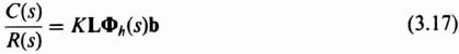
Substituting Eq. (3.15) into Eq. (3.12), we obtain a relation between C(s) and R(s):

Therefore, the closed-loop transfer function in terms of the closed-loop resolvent matrix is given by

In addition, the characteristic equation in terms of the closed-loop-system matrix can also easily be determined, simply by substituting the numerator and denominator portions of the inverse matrix, Φ_h(s):

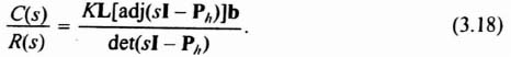
The corresponding characteristic equation of the closed-loop system in terms of the closed-loop system matrix is given by

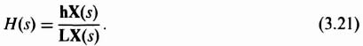
Because we are concerned with synthesizing control systems in terms of pole placement design using linear-state-variable feedback concepts, we would like to force the system illustrated in Figure 3.3 into the generalized form illustrated in Figure 3.5, and study its properties. Let us first consider the derivation of H(s). From Figure 3.5 we observe that

Substituting Eq. (3.12) into Eq. (3.20), we obtain

After substitution of Eq. (3.15) for X(s), Eq. (3.21) becomes

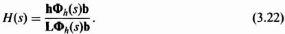
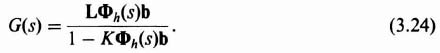
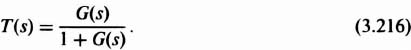
The term G(s) can also be derived in terms of Φ_h(s). The closed-loop transfer function of the system illustrated in Figure 3.5 is given by

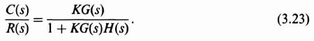
Substituting Eqs. (3.17) and (3.22) into Eq. (3.23), we obtain the expression

Combining Eqs. (3.22) and (3.24), the open-loop transfer function is found to be given by

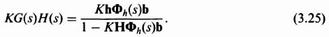
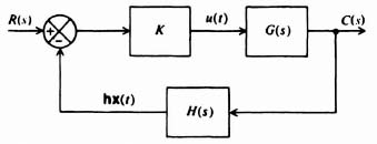
Figure 3.5 An equivalent model of Figure 3.3.

Let us compare Eqs. (3.17), (3.22)–(3.24), and (3.25) in order to draw conclusions regarding G(s), H(s), the open-loop transfer function KG(s)H(s), and the closed-loop transfer function C(s)/R(s). These characteristics will be important for designing systems using pole placement techniques with linear-state-variable feedback techniques in the following section. Based on these five equations, we can state the following properties:

1. The poles of KG(s)H(s) are the poles of G(s).
2. The zeros of C(s)/R(s) are the zeros of G(s).
3. The pole-zero excess of C(s)/R(s) must be equal to the pole-zero excess of G(s).

With these properties as a basis, we consider in the following section the design of control systems from the viewpoint of linear-state-variable feedback.

3.3. CONTROLLER DESIGN USING POLE PLACEMENT AND LINEAR-STATE-VARIABLE FEEDBACK TECHNIQUES

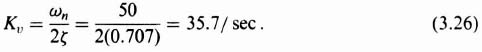
The preceding section has indicated several important relationships between open-loop and closed-loop transfer functions. This is very important in the design of control systems for the case where the closed-loop transfer function is specified and it is desired to determine the open-loop transfer function. A typical problem might specify the desired velocity constant; then use is made of Eq. (C.29) in Appendix C which gave the velocity constant in terms of the closed-loop poles and zeros. The problem is to determine the resulting linear-state-variable feedback system.

Let us illustrate the procedure by considering the following problem. It is desired that the closed-loop characteristics of a unity-feedback control system be given by the following parameters:

What form of closed-loop transfer function will satisfy these requirements? Let us first try a simple quadratic control system having a pair of complex-conjugate poles. From Eq. (C.31) of Appendix C, such a system has a velocity constant given by

Therefore, a simple quadratic control system having a pair of complex-conjugate poles will satisfy these specifications. From Eq. (B.18) of Appendix B,

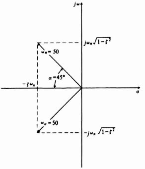
For a damping ratio of 0.707, α = 45° and the relations among the complex-conjugate poles, ω_n and ζ are illustrated in Figure 3.6. Therefore, the closed-loop control system is given by

Figure 3.6 Closed-loop poles.

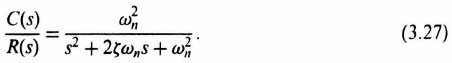
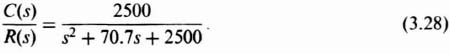
By substituting ζ = 0.707 and ω_n = 50 into Eq. (3.27), we obtain the following desired closed-loop transfer function:

Let us assume that the open-loop process that is being controlled is illustrated in Figure 3.7. The corresponding state-variable representation is readily found to be

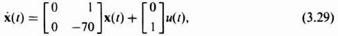
where

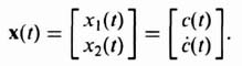
The resulting linear-state-variable feedback representation is illustrated in Figure 3.8. This feedback represenation can be simplified by the configuration illustrated

Figure 3.7 Open-loop process to be controlled.

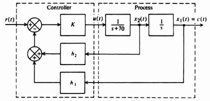
Figure 3.8 State-variable feedback representation of system.

in Figure 3.9. The resulting closed-loop transfer function is given by

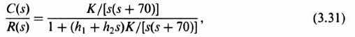
which can be reduced to the following expression:

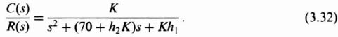
The values of K₁h₁, and h₂ can be found from Eqs. (3.28) and (3.32). The following set of simultaneous equations result:

We have three equations and three unknowns. Solving, we find that h₁ = 1, K = 2500, and h₂ = 2.8 × 10⁻⁴. The final step is to draw the root locus and examine the relative stability, and the sensitivity as a function of slight gain variations. For this simple system, the final step is not necessary.

Although this simple example has been solved using block diagrams and transfer functions, it could also have been solved using the matrix-algebra approach. To illustrate this, let us pick up this problem from Eq. (3.28) which is the desirable closed-loop transfer function. We want to determine the closed-loop transfer function

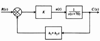
Figure 3.9 Equivalent configuration of Figure 3.8.

for the linear-state-variable-feedback control system using Eq. (3.18) and knowledge of the P and B matrices from Eq. (3.29), and the matrix L from Eq. (3.30) as follows:

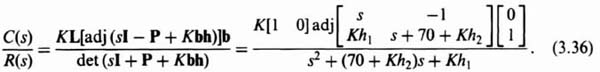
Simplifying Eq. (3.36), we obtain the following:

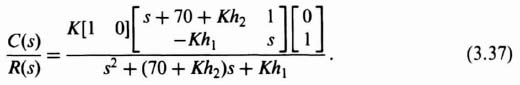
Simplifying Eq. (3.37) results in the following expression for the closed-loop transfer function of the system:

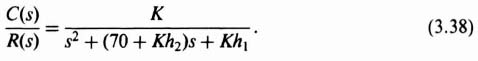
Equation (3.38) is identical to the closed-loop transfer function we obtained in Eq. (3.32) which was obtained from the block diagram shown in Figure 3.8. Therefore, we repeat the process of setting like terms equal to each other from Eq. (3.38) and Eq. (3.28). The resulting three simultaneous equations of (3.33) through (3.35) will be identical, and the resulting parameters of K = 1, h₁ = 1, and h₂ = 2.8 × 10⁻⁴ will be the same as found before.

With this fundamental example as a basis, the general pole placement design procedure can be formulated as follows:

1. Determine the desired closed-loop transfer function based on the discussion of Appendix C.
2. Determine the representation of the process to be controlled.
3. Represent the closed-loop system in terms of an equivalent linear-state-variable-feedback configuration.
4. Determine the closed-loop transfer function C(s)/R(s) from the equivalent model in terms of K and h.
5. Equate the C(s)/R(s) expressions from Steps 1 and 4 and determine K and h.*
6. Plot the resulting root locus of KG(s)H(s) and evaluate the relative stability and sensitivity as a function of gain variations.

Let us apply this pole placement procedure next to the following more complex example. The problem concerns the control of a process in a unity-feedback closed-loop system whose transfer function is given by

It is assumed that the transient response of the system is governed by a pair of dominant complex-conjugate poles, and that the following parameters are desired:

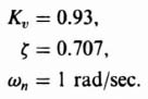
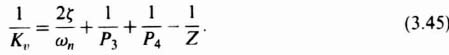
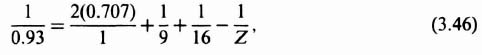
What should the closed-loop transfer function be? From Eq. (3.26), a pair of complex-conjugate poles in the denominator would only have a velocity constant given by

Therefore, a simple pair of complex-conjugate poles is inadequate to meet the velocity constant requirement of 0.93. By examining Eq. (C.29), we conclude that a zero Z must be added to the closed-loop transfer function. How many poles should the closed-loop system have? Because

where

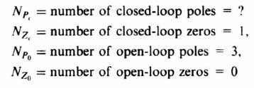
therefore,

and

Since the resulting unity-feedback, closed-loop transfer function has to have one zero and four poles, it has the following general form: The value of the zero Z can be found from Eq. (5.35) as follows:

The value of the zero Z can be found from Eq. (5.35) as follows:

Due to external overall system factors in which this feedback system is to operate, it is assumed that the poles at P₃ and P₄ are specified to occur at 9 and 16, respectively. Therefore,

so that Z = 2, and the desired closed-loop transfer function is given by

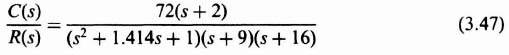
or

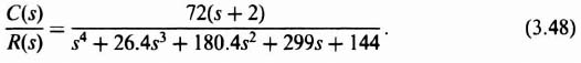
Because the zeros of G(s) must be the same as that of C(s)/R(s), we must also add the factor (s + 2) to the numerator of G(s). Then, to satisfy Eq. (3.41), we must add a pole factor (s + α) to the denominator of G(s). The resulting compensating network to be added to G(s) is given by

where α is a pole of the open-loop transfer function which is to be determined. The resulting linear-state-variable feedback system is illustrated in Figure 3.10. The problem remaining is to select the values of K, α, and h.

Figure 3.10 State-variable feedback representation of system.

An equivalent block diagram of this system is illustrated in Figure 3.11. The resulting closed-loop transfer function from this equivalent model is given by

Equating the two forms of C(s)/R(s) given by Eqs. (3.48) and (3.50), the following set of equations is obtained:

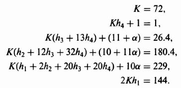
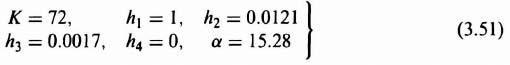
Notice that we have six simultaneous equations with six unknowns (K, h₁, h₂, h₃, h₄, and α). Solving these equations, we obtain the following expressions:

From Eq. (3.49), the resulting compensation network, G_c(s), is given by

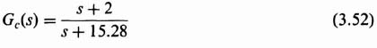
which is a phase-lead network.

It is important to emphasize that α could have turned out to be negative for a different set of specifications This would be undesirable, because it would result in a zero in the right-half plane; this system would be unstable. In other cases, the system might be conditionally stable.

Our results of this pole placement example can be evaluated most conveniently on a root-locus plot. To obtain the root locus of the compensated system, the open-loop

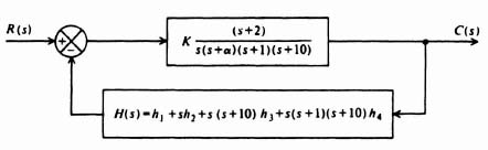
Figure 3.11 Equivalent block diagram for system illustrated in Figure 3.10.

transfer function will be obtained. For the values of the parameters found in Eq. (3.51), H(s) results in the following:

Combining Eqs. (3.39), (3.52), and (3.53) we obtain the following transfer function for the open-loop system:

The resulting root locus is plotted in Figure 3.12. Observe that the resulting root locus is stable for all values of K from zero to infinity. The locations of the dominant complex-conjugate roots for K = 72 are indicated.

It is important to emphasize again that the discussion of linear-state-variable feedback in this and the preceding section has assumed that all of the state variables are accessible. This is not always the case. This is analyzed further in Sections 3.6 and 3.7.

3.4. CONTROLLABILITY

The presentation of linear-state-variable feedback in Sections 3.2 and 3.3 assumed that all of the states are observable and measurable, and available to accept control signals (controllable). The concepts of controllability [2–4], and observability also playa very important role in optimal control theory (presented in the accompanying volume). Before designing a control system, we must determine whether it is controllable and its states are observable, since the conditions on controllability and observability often govern the existence of a solution to an optimal control system. Kalman [2,3] first introduced the concepts of controllability and observability in 1960. These concepts are basic in modern optimal control theory. This section develops mathematical tests to determine controllability, and the following section presents mathematical tests for determining observability.

Figure 3.12 Root locus for the system of Figure 3.11 with the parameters of Eq. (3.51)

In order to introduce the concept of controllability, let us consider the simple open-loop system illustrated in Figure 3.13. A system is completely controllable if there exists a control which transfers every initial state at t = t₀ to any final state at t = T for all t₀, and T. Qualitatively, this means that the system G(s) is controllable if every state variable of G can be affected by the input signal u(t). However, if one (or several) of the state variables is (or are) not affected by u(t), then this (or these) state variable(s) cannot be controlled in a finite amount of time by u(t) and the system is not completely controllable.

A. Controllability by Inspection

As an example of a system which is not completely controllable, let us consider the signal-flow diagram illustrated in Figure 3.14. This system contains four states, only two of which are affected by u(t). This input only affects the states x₁(t) and x₂(t). It has no effect on x₃(t) and x₄(t). Therefore, x₃(t) and x₄(t) are uncontrollable. This means that it is impossible for u(t) to change x₃(t) from initial state x₃(0) to final state x₃(T) in a finite time interval T and the system is not completely controllable.

B. The Controllability Matrix

Let us now consider this problem more precisely and establish a mathematical criterion for determining whether a system is controllable. We limit our discussion to linear constant systems. Assume that the system is described by

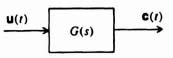
Figure 3.13 Open-loop system containing several inputs and outputs.

Figure 8.14 Signal-flow graph of a system that is not completely controllable.

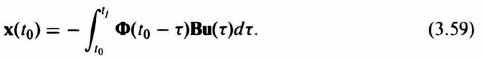
The solution of Eq. (3.55) can be expressed as Eq. (2.265)^‡:

Let us assume that the desired final state of our system at t = t_f is zero:

Using Eqs. (2.259)^‡ and (2.261)^‡, we can write Eq. (3.57) as

The state-transition matrix can be expressed from Eq. (2.322)^‡ as

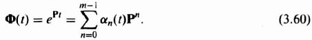
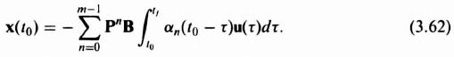
Here, x is an m × 1 vector, P is an m × m matrix, u is an r × 1 vector, B is an m × r matrix, and α_n(t) is a scalar function of t. (This form results from application of the Cayley–Hamilton theorem). Substituting Eq (3.60) into Eq. (3.59), we obtain the following expression for x(t₀):

Because the matrices P and B are not functions of τ, we can rewrite Eq. (3.61) as

Equation (3.62) can be rewritten as

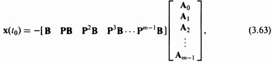
where

If we define

where D, the controllability matrix, is an m × mr matrix and A is an mr × 1 vector, then Eq. (3.63) becomes

For a given initial state x(t₀), the input u can be found to drive the state to x(t_f) = 0 for a finite time interval t_f − t₀ if Eq. (3.67) has a solution. A unique solution occurs only if there is a set of m linearly independent column vectors in the matrix D. If u is a scalar, then D is an m × m square matrix, and Eq. (3.67) represents a set of m linearly independent equations which have a solution if D is nonsingular or the determinant of D is not zero. The controllability criterion thus states that the system of Eqs. (3.55) and (3.56) is completely controllable if D [see Eq. (3.65)] contains m linearly independent column vectors or, if u is a scalar, D is nonsingular.

In order to illustrate this mathematical controllability concept, consider a second-order system where

and

Then, from Eq. (3.65),

The resulting matrix D is singular (its determinant is zero) and the system is therefore not completely controllable.

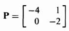
As a second example, consider a second-order system where

and

Then, from Eq. (3.65)

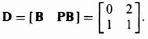
The resulting matrix D is nonsingular and the system, therefore, is completely controllable.

3.5. OBSERVABILITY

In order to introduce the concept of observability [2–4], let us again consider the simple open-loop system illustrated in Figure 3.13. A system is completely observable if, given the control and the output over the interval t₀ t T, one can determine the initial state x(t₀). Qualitatively, the system G is observable if every state variable of G affects some of the outputs in c. It is very often desirable to determine information regarding the system states based on measurements of c. However, if we cannot observe one or more of the states from the measurements of c, then the system is not completely observable. We had assumed the systems were observable in our discussion of pole placement using linear-state variable feedback in Sections 3.2 and 3.3.

A. Observability by Inspection

As an example of a system which is not completely observable, let us consider the signal-flow diagram illustrated in Figure 3.15. This system contains four states, only two of which are observable. The states x₃(t) and x₄(t) are not connected to the output c(t) in any manner. Therefore, x₃(t) and x₄(t) are not observable and the system is not completely observable.

B. The Observability Matrix

Let us now consider this problem more precisely and establish a mathematical criterion for determining whether a system is completely observable. Again, we limit our discussion to linear constant systems of the form

where x is an m × 1 vector, P is an m × m matrix, u is an r × 1 vector, B is an m × r matrix, c is a p × 1 vector, and L is a p × m matrix. The solution of Eq. (3.69) is given by [see Eq. (3.57)]

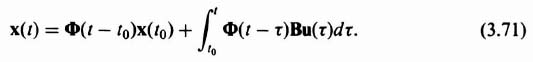
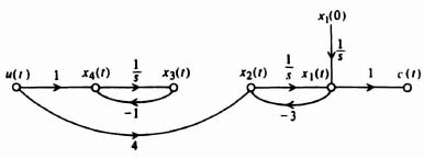
Figure 3.15 Signal-flow graph of a system that is not completely observable.

It will now be shown that observability depends on the matrices P and L. Substituting Eq. (3.71) into Eq. (3.70), we obtain

From the definition of observability we can see that the observability of x(t₀) depends on the term LΦ(t − t₀)x(t₀). Therefore, the output c(t) when u = 0 is given by

Substituting Eq. (3.60) into Eq. (3.73), we obtain the following expression for the output c(t):

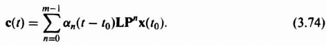
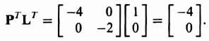
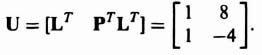
Equation (3.74) indicates that if the output c(t) is known over the time interval t₀ t T, then x(t₀) is uniquely determined from this equation if x(t₀) is a linear combination of (L_jPⁿ)^T for n = 0, 1, 2, …, m − 1, and j = 1, 2, 3,…, r. The matrix L_j is the 1 × m matrix formed by the elements of the jth row of L. Because , we let U be the m × mr matrix defined by

The observability criterion states that the system is completely observable if there is a set of m linearly independent column vectors in the observability matrix U.

In order to illustrate the observability concept mathematically, consider a second-order system where

and

Therefore,

and

Substituting these values into Eq. (3.75), we obtain

Because U is singular, the system is not completely observable.

As a second example, consider the second-order system where

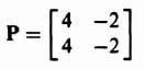
and

Therefore,

and

Substituting these values into Eq. (3.75), we obtain

Because U has two independent columns, the system is completely observable.

3.6. ACKERMANN'S FORMULA FOR DESIGN USING POLE PLACEMENT [5–7]

In addition to the method of matching the coefficients of the desired characteristic equation with the coefficients of det (sI − P_h) as given by Eq. (3.19), Ackermann has developed a competing method. The pole placement method using the matching of coefficients of the desired characteristic equation with the coefficients of Eq. (3.19) is very useful for control systems which are represented in phase-variable form, where phase variable refers to systems where each subsequent state variable is defined as the derivative of the previous state variable. Some control systems require feedback from state variables which are not phase variables. Such high-order control systems can lead to very complex calculations for the feedback gains. Ackermann's method simplifies this problem by transforming the control system to phase variables, determining the feedback gains, and transforming the designed control system back to its original state-variable representation.

Let us represent a control system which is not represented in phase-variable form by the following:

We will assume that the controllability matrix [see Eq. (3.65)] can be represented by

Subscript y is used to designate the original, non-phase-variable, controllability matrix. We will next assume that the control system can be transformed into the phase-variable representation using the following transformation:

Substituting Eq. (3.79) into Eq. (3.76) and Eq. (3.77), we obtain:

Using the transformation of Eq. (3.79), the controllability matrix for the transformed system defined by Eqs. (3.80) and (3.81) is:

The subscript x is used to designate the phase-variable form of the transformed control system. Equation (3.82) can be simplified to

Therefore, substituting Eq. (3.78) into Eq. (3.83), we find that

The transformation matrix A can be found from

Therefore, the transformation matrix A can be determined from the controllability matrices defined by Eqs. (3.65) and (3.83). Once the control system is transformed to the phase-variable form, the feedback gains h can be determined as described in Section 3.2.

Returning to Eq. (3.4) to represent u(t) for the control system in phase-variable form,

the following is obtained by substituting Eq. (3.86) into Eq. (3.80):

Equation (3.87) can be simplified to the following phase-variable state equation:

The output equation remains as shown in Eq. (3.81):

Because Eqs. (3.88) and (3.89) are in phase-variable form, the rules for pole placement developed in Section 3.2 for phase-variable systems are valid for this representation. We now have to transform Eqs. (3.88) and (3.89) back to the original state and output equation representation by using the transformation provided by Eq. (3.79):

Substituting Eq. (3.90) into Eq. (3.88), we obtain the following:

Therefore, Eq. (3.91) reduces to the following state equation:

The output equation is found by substituting Eq. (3.79) in Eq. (3.89):

By comparing Eq. (3.92) with Eqs. (3.8) and (3.10), we find that the state-variable feedback constants for the original system are

A. Example Applying Ackermann's Formula for Design using Pole Placement

We wish to apply the pole placement concepts using Ackermann's design formula to a system that uses linear-state-variable feedback. The system specifications require an overshoot of 4.33% and a settling time of 6 sec. The process transfer function is

and the control system's signal-flow graph is given in Figure 3.16.

The state equation for the process illustrated in Figure 3.16 is:

Since we are going to need the controllability matrix D_y to convert this original system to phase-variable form [see Eq. (3.85)], let us compute this controllability matrix for this original system:

The value of the determinant of D_y is −1, it is nonsingular, and the original control system is controllable as expected from inspection of Figure 3.16.

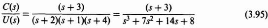
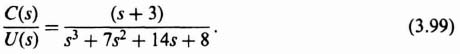
The next step is to transform the original system to the phase-variable form. This can easily be obtained from the transfer function C(s)/U(s), which can be determined from Figure 3.16:

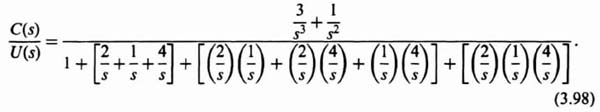
Eq. (3.98) can be reduced to the following [as stated in Eq. (3.95)]:

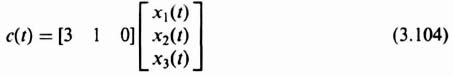
We can determine the phase-variable state equations which represent the transfer function given by Eq. (3.99). Defining x₁(t) = c(t), x₂(t) = c(t), and x₃(t) = , we obtain the following:

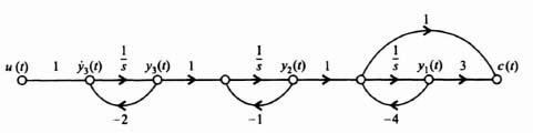
Figure 3.16 Signal-flow graph representation of process whose transfer function is defined in Eq. (3.95).

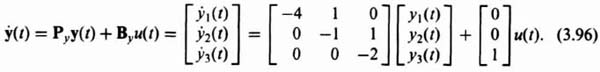
Therefore, the state and output equations in matrix vector form of the phase-variable control system are given by:

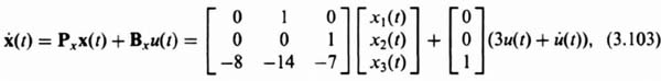
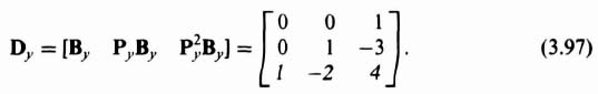
The resulting controllability matrix for the phase-variable form can be obtained from Eqs. (3.65) and (3.103) and is given by:

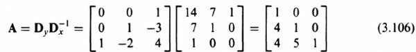
Note that the determinant of D_x is −1 indicating that the determinant is nonsingular, and the phase-variable form is also controllable, as expected. The transformation matrix, defined in Eq. (3.85), can be determined from Eqs. (3.97) and (3.105) as follows:

The next step in the procedure is to design the controller (see Figure 3.3) using the phase-variable representation, after which we will transform the design back to the original system by using Eq. (3.106). The 4.33 percent overshoot specified can be obtained from a second-order control system having a damping ratio of 0.707 [see Eq. (B.33)]. The settling time of 6 sec can be obtained from a second-order control system having a damping ratio of 0.707 and ω_n = 0.943 [see Eq. (5.41)^‡]. Therefore, the following second-order control system can meet the design specifications:

Since it was shown in Section 3.2 that zeros of closed-loop systems are zeros of open-loop systems, then we can select the third pole at s = −3 which will also cancel the zero at s = −3. Therefore, the characteristic equation of the desired closed-loop system is

The state and output equations for the phase-variable form with linear-state-variable-feedback can be obtained from Eqs. (3.8), (3.9), and (3.10) as follows:

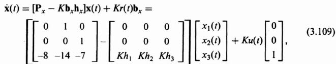
Eq. (3.109) reduces to the following:

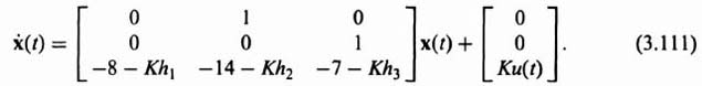
The resulting characteristic equation can be obtained from Eqs. (3.10) and (3.19):

Substituting −(P_x − Kb_xh_x) from Eq. (3.111) into Eq. (3.112), we obtain the following:

The resulting characteristic equation is given by:

Comparing Eq. (3.114) and Eq. (3.108), we obtain the following three equations:

Therefore,

We will now transform Kh_x as shown in Eq. (3.118) back to the original system using Eq. (3.94) and Eq. (3.106) as follows:

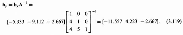
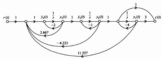
Figure 3.17 Resulting closed-loop control system with linear-state-variable-feedback designed using Ackermann's Formula.

The resulting closed-loop control system with linear-state-variable-feedback is shown in Figure 3.17.

3.7. ESTIMATOR DESIGN IN CONJUNCTION WITH THE POLE PLACEMENT APPROACH USING UNEAR-STATE-VARIABLE FEEDBACK

In the discussion of Sections 3.2 and 3.3 on linear-state-variable feedback, it was assumed that all of the states are observable and measurable, and available to accept control signals (controllable). As Sections 3.4 and 3.5 on controllability and observability have shown, some states of a feedback control system may not always be controllable and/or observable. In some systems, the system may be observable, but all of the states may not be measured due to physical limitations (e.g., chemical process control systems), or it may be due to cost restrictions that limit the use of costly sensors needed to measure all of the states. It is assumed in this section that the system is observable (no part of the system is disconnected physically from the output), but measurements are being made only on some of the states, and we wish to estimate all of the states.

Let us focus attention on the process portion of the system illustrated in Figure 3.3. We wish to use the closed-loop estimator system shown in Figure 3.18 for determining an estimate of the state vector x(t) and output c(t) [8]. This estimator feeds back the difference between the measured output c(t) and the estimated output c(t) that is obtained from a model of the process. Therefore,

where M defines the gain factors m_i, which are selected to obtain desirable error characteristics of the state vector x, and represents the estimate of the state x(t):

The error in the state estimate, , can be derived from

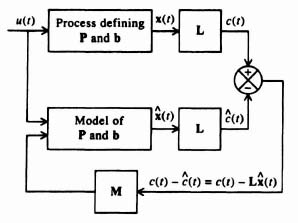
Figure 3.18 An estimator system.

The derivative of the can be obtained by subtracting [given by Eq. (3.120)] from given by the system dynamics:

Subtracting Eq. (3.120) from Eq. (3.123), we obtain the following:

Substituting Eq. (3.2),

into Eq. (3.126), we obtain

Using the definition of error in the state estimate as given by (3.122), Eq. (3.128) reduces to

or

It is shown in Section 6.2^‡ on the state-variable determination of the characteristic equation that a state equation, as given by Eq. (6.15)^‡,

has a characteristic equation given by Eq. (6.22)^‡. Similarly, the characteristic equation of Eq. (3.129) is given by

The objective of the control-system engineer is to select P – ML so that it has stable roots in order for to decay to zero. It is also desirable to have the root location produce a fast transient response so that the estimation error decays very fast to zero. Notice that the estimation error will converge to zero independent of the forcing function u(t). Therefore, stability is determined from the homogeneous solution to the system (with u(t) = 0), as opposed to its particular solution (with u(t) finite).

The design procedure for determining M is to specify the desired location of the estimator roots (e.g., α₁, α₂,…, α_n) from which the desired estimator characteristic equation can be specified:

We can then solve for M by comparing the coefficients in Eqs (3.131) and (3.132).

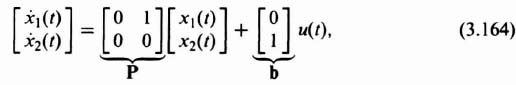
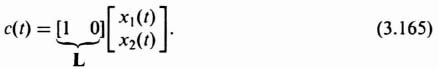
Let us consider the design of M for a simple second-order system whose differential equation is given by

Defining its two states as

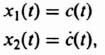
we obtain its state equations as

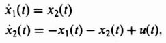
and its output equation as

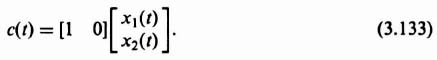
Therefore, for this system, we obtain P, b, and L to be as follows:

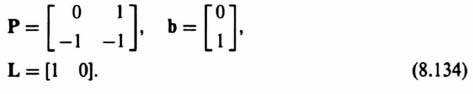
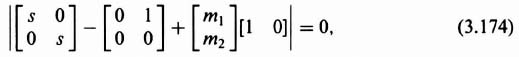
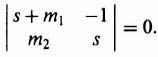
Substituting Eq. (3.134) into Eq. (3.131), we obtain the following:

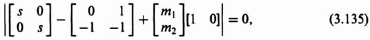
The resulting characteristic equation is given by

Where do we desire to place the two second-order roots? The primary goal is to design the estimator to be very fast compared to that of the controller. Therefore, let us assume that the controller is critically damped and the controller's second-order characteristic equation has a pair of real roots located at s = β₁ = β₂ = 2. Let us assume that we wish the estimator to be critically damped and have the two second-order roots of the estimator located at s = α₁ = α₂ = 20 in Eq. (3.132), which will ensure a very fast response compared to that of the controller. Therefore, Eq. (3.132) for this example becomes

Comparing the coefficients of Eqs. (3.138) and (3.139), we obtain the following two sumultaneous equations to solve:

Solving Eqs. (3.140) and (3.141), we obtain:

Designing a combined compensator of a controller and estimator is illustrated in Section 3.8.

3.8. COMBINED COMPENSA FOR DESIGN INCLUDING A CONTROLLER AND AN ESTIMATOR FOR A REGULATOR SYSTEM

This section considers the combined compensator design of a controller and estimator for a regulator in which the reference input equals zero, and for the case where the reference input is finite. The block diagram of this regulator is shown in Figure 3.19, which combines the concepts illustrated in Figure 3.3 for the controller and Figure 3.18 for the estimator. We wish to determine in this system the effect of using the estimated state vector , instead of x(t) on the system dynamics [8].

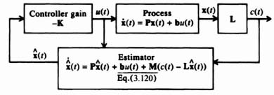
Figure 3.19 Regulator system (where the reference input r = 0) containing combined controller and estimator.

Let us consider the effect of driving the controller with instead of x(t). From the process dynamics shown in Figure 3.3,

From Figure 3.19, we also know that

Therefore, substituting Eq. (3.143) into Eq. (3.142), we obtain

In terms of the state estimation error defined in Eq. (3.122), Eq. (3.144) becomes

Combining Eqs. (3.145) and (3.129), we obtain an overall equation for the state vector x and its error as follows:

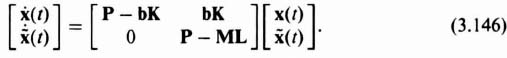
The characteristic equation of this closed-loop combined controller and estimator system can be obtained in a manner similar to that obtained for the estimator alone [see Eq. (3.131)]:

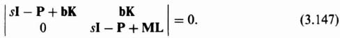
We can write this equation as

The first determinant specifies the characteristic equation of the controller, and the second determinant specified the characteristic equation of the estimator [which is identical to Eq. (3.131)]. As we did for the case of the estimator alone in Section 3.7, Eq. (3.132), we can now define the combined desirable location of estimator roots

and controller roots

and specify the combined estimator and controller's characteristic equation as

We can now simultaneously determine the controller gain K and estimator coefficients M by setting Eqs. (3.148) and (3.149) equal to each other:

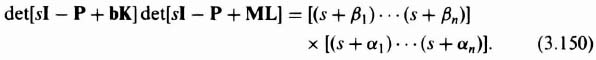
Therefore, we can observe from Eq. (3.150) that the roots of the combined controller and estimator is the sum of the controller and estimator roots found independently [8]. The primary concept to recognize in the combined compensator design for the controller and estimator is to make the estimator respond much faster than the controller, as we do not want the system's transient response limited by that of the estimator (which we can control by proper design).

It is useful to compare the modern pole placement method using the state-variable feedback method with the conventional transfer-function method for the design of the compensator as we have done in Section 3.2, when we found the open-loop transfer function KG(s)H(s) in terms of h, Φ_h(s) and b in Eq. (3.25). We wish to find the transfer function of the combined controller and estimator, U(s)/C(s). Let us reconsider the estimator equation, Eq. (3.120), and incorporate it in the control-law equation, Eq. (3.143), because the controller is part of the compensator:

Simplifying, we obtain

Let us compare Eq. (3.152) with the state equation of the process:

whose characteristic equation we know is given by

using the same reasoning we used in obtaining Eqs. (6.22)^‡, (3.19), and (3.131). By comparing Eqs. (3.152) and (3.153), we obtain the characteristic equation of the compensator as follows:

The resulting compensator may not result in a stable system because the roots of Eq. (3.155) have not been specified in advance. This is similar to our results in Section 3.3, where we found that design using linear-state-variable feedback did not ensure a stable system.

Before finding the transfer function representing the compensator, U(s)/C(s), we first find the transfer function of the process from Eq. (3.153):

Simplifying,

Solving for X(s), we obtain

Since

and its Laplace transform is

we can combine Eqs. (3.158) and (3.159) to relate the output C(s) and input U(s) of the process.

In order to find the transfer function of the process C(s)/U(s), we assume that the initial condition, x(0), equals zero. Therefore,

By analogy, we compare Eqs. (3.153) [and its resulting transfer function given by Eq. (3.161)] with Eq. (3.152), and conclude that the transfer function of the compensator defined by Eq. (3.152) is given by

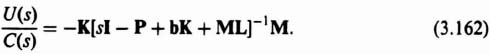
When we determine the transfer function U(s)/C(s) using this procedure, we will find that the resulting transfer function will result in a phase-lead network, a phase-lag network, or a phase-lag-lead network.

To illustrate this approach for obtaining the transfer function of the compensator, consider a process whose transfer function is given by

Therefore,

Defining the state variables of this second-order system as

we obtain the state equation to be

and the output equation is

Let us assume that the design specification for the controller is

Therefore, the complex-conjugate roots of the controller are located at −1 ± j1.414 and a_c(s) for the controller is given by

We can determine the controller gain K by equating like powers of s from Eq. (3.166) and that part of Eq. (3.148) concerned with the controller:

Substituting for P and b from Eq. (3.164) into Eq. (3.167), we obtain the following:

This simplifies to

from which we obtain the characteristic equation of the controller:

Comparing like coefficients in Eqs. (3.166) and (3.170), we find the controller gains to be K₁ = 3 and K₂ = 2:

As discussed previously, we desire the estimator to have a much faster response than the controller. Therefore, let us assume the design specification of the estimator to be

Therefore, the complex-conjugate roots of the estimator are located at −8.5 ± j14.7, and α_e(s) for the estimator is given by

The resulting estimator feedback gain matrix is found from Eq. (3.131) [for the estimator portion of Eq. (3.148)] as follows:

Substituting the matrix values into Eq. (3.173), we obtain

which reduces to:

The resulting characteristic equation in terms of m₁ and m₂ is given by

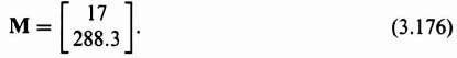
Setting like coefficients in Eqs. (3.172) and (3.175) equal to each other, we obtain m₁ = 17 and m₂ = 288.3:

The resulting compensator transfer function is obtained by substituting parameters obtained from Eqs. (3.164), (3.165), (3.171), and (3.176) into Eq. (3.162) as follows:

This equation reduces to

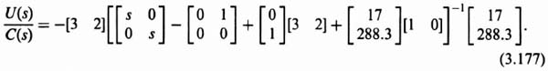
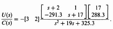
Upon further simplification, we obtain the following:

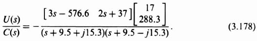
The resulting transfer function of the compensator is given by the following equation:

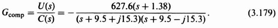
Analysis of Eq. (3.179) shows that the compensator has the form of a phase-lead network with a zero at −1.38 and with two complex-conjugate poles as opposed to a simple pole as defined by the conventional phase-lead network of Eq. (2.6).

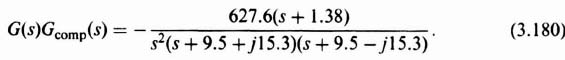
We can analyze the resulting system using the conventional root-locus and Bode-diagram methods. To obtain the open-loop transfer function for analyses, we combine Eqs. (3.163) and (3.179):

Replacing the specific gain of −627.6 with the variable gain K, the root locus can be evaluated from

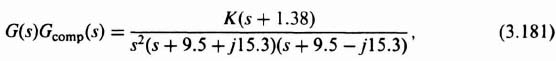
which is shown in Figure 3.20. Observe that the root locus goes through the roots chosen in Eqs. (3.166) and (3.172) when K = 627.6. These roots are shown in Figure 3.20 by solid dots. This figure was obtained using MATLAB, and is contained in the M-file that is part of my AMCSTD Toolbox which can be retrieved from The MathWorks anonymous FTP server at ftp://ftp.mathworks.com/pub/books/advshinners.

To draw the Bode diagram, we consider the modified form of Eq. (3.180):

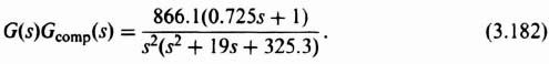
The resulting Bode diagram is drawn from the following simplification to Eq. (3.182):

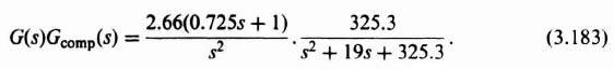
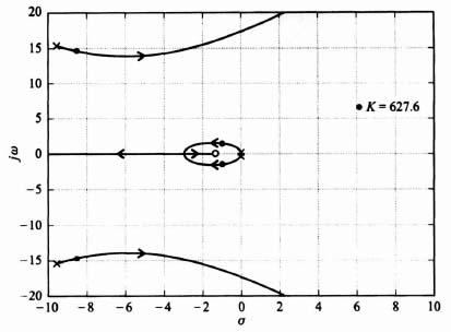
Figure 3.20 Root locus for compensated system of Figure 3.19 where G(s)G_comp(s) = (K(s + 1.38))/(s²(s + 9.5 + j15.3)(s + 9.5 − j15.3)).

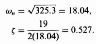
The quadratic poles in the denominator have an undamped natural frequency ω_n and a damping ratio ζ given by

The resulting Bode diagram is shown in Figure 3.21. This figure was also obtained using MATLAB and is contained in the M-file that is part of my AMCSTD Toolbox.

We conclude that the uncompensated transfer function

has its phase margin increased from 0 to 51.07 degrees at its gain crossover frequency of 2.28 rad/sec., and its gain margin is increased from minus infinity to 19.13 dB (phase crossover frequency occurs at ω = 17.32 rad/sec) when we use the compensator of Eq. (3.179). Notice that the crossover frequency of 2.28 rad/sec is approximately consistent with the controller's closed-loop roors of rad/sec and ζ = 0.85. This is a reasonable result, as the slower roots of the controller are more dominant than the faster estimator roots, on the system response.

A complete case study for the design of a combined controller and estimator for a regulator, using the techniques presented in Section 3.7 and 3.8, is presented in Chapter 7.

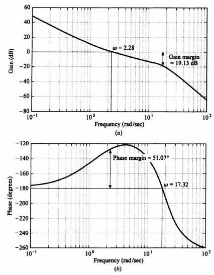
Figure 3.21 Bode diagram for compensated system of Figure 3.19 where G(s)G_comp(s) = ((2.66(0.725s + 1))/s²)(325.3/(s² + 19s + 325.3)).

3.9. EXTENSION OF COMBINED COMPENSATOR DESIGN INCLUDING A CONTROLLER AND AN ESTIMATOR FOR SYSTEMS CONTAINING A REFERENCE INPUT

How can we extend the concepts developed in the previous section for regulator design, shown in Figure 3.19 (where the reference input r(t) = 0), to the more general problem where the reference input exists? Several methods exist which can be used to design such a system [8,9]. This section will consider the configuration illustrated in Figure 3.22. The design goal of the approach to be presented is to have the state-estimation error be independent of the reference input r(t) (e.g., should be uncontrollable from r(t)). This is a very important consideration, as we do not want the state-estimation error to be dependent on the type and level of the input.

Let us reconsider the controller equation (3.143),

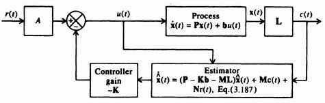
Figure 3.22 Addition of the reference input to the system shown in Figure 3.19 containing a combined controller and estimator.

and the estimator equation (3.152)

The reference input r(t) will be introduced to these equations by adding a term Ar(t) to the controller equation (3.184), and a term Nr(t) to the estimator equation (3.185) (where N is a vector). Therefore, Eqs. (3.184) and (3.185) become

What kind of system do Eqs. (3.186) and (3.187) infer? Does it result in the configuration of Figure 3.22? To answer this question, let us first substitute

into Eq. (3.187) and, thereby, eliminate the output c(t) from Eq. (3.187):

To find the estimation error (which we want to be independent of r(t)), let us difference [from Eq. (3.189)] and the state equation

We will first substitute Eq. (3.186) into Eq. (3.190):

Subtracting Eq. (3.189) from Eq. (3.191), we obtain the following for the derivative of the estimation error:

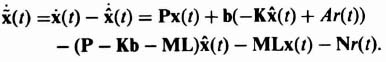
Simplifying, we obtain the following equation:

In order to eliminate r(t) from Eq. (3.192), it is necessary that

Therefore, the design criterion of the control-system engineer is to invoke Eq. (3.193). Substituting Eqs. (3.186) and (3.193) into Eq. (3.187), we obtain the following:

Simplifying, we find that

or

Notice that Eq. (3.196) is the same estimator equation defined in Eq. (3.120). It is important to emphasize that this occurs only when bA = N as defined in Eq. (3.193). Therefore we conclude that the introduction of the reference input by adding the term Ar(t) in the controller equation (3.186) and a term Nr(t) to Eq. (3.187) results in the configuration shown in Figure 3.22.

Complete design examples for the design of the controller, estimator, and compensator, with their associated root-locus and Bode-diagram analyses of the resulting design are found in Chapter 7. In Section 7.5, the state-variable design for the controller and full-order estimator for a space vehicle is presented. In Problem 7.6, the state-variable design for the controller and full-order estimator of a chemical process control system is analyzed.

3.10. ROBUST CONTROL SYSTEMS [10–14]

Robust control is concerned with determining a stabilizing controller that achieves feedback performance in terms of stability and accuracy requirements, but the control must achieve the performance that is robust (insensitive) to plant uncertainty, parameter variation, and external disturbances. We know from the previous discussion in this book that feedback reduces the effects of external disturbances (Section 1.7) and parameter variations (Section 1.7). However, this is only achieved with relatively high loop gain which limits stability. Robust control is basically the same problem that was addressed in the 1930s by Black, Bode, and Nyquist. Modem robust control revolves around the feedback configurations illustrated in Figures 2.5, 2.6, and 2.7 which illustrate two-degrees-of-freedom compensation systems.

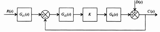
Figure 3.23 Control system with a two-degrees-of-freedom series controller G_c1(s) and a forward-loop-controller G_c2(s).

Let us consider the control system illustrated in Figure 3.23 which contains a disturbance D(s), and it contains a two-degrees-of-freedom series controller G_c1(s) and a forward-loop controller G_c2(s). In this control system's operation, the amplifier gain, K, can vary.

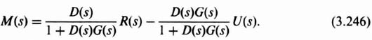
For this control system, the overall transfer function, C(s)/R(s), is given by

The transfer function relating the disturbance D(s) to the output C(s) is given by

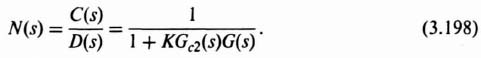
The design approach in robust control systems is to choose the controller G_c1(s) so that the desired closed-loop transfer function H(s) is obtained, and to choose the controller G_c2(s) so that the output, C(s), is insensitive to the disturbance D(s) over the frequency range in which D(s) is dominant.

The sensitivity of H(s) due to variations of K is given by

For the control system of Figure 3.23,

Substituting Eqs. (3.197) and (3.200) into Eq. (3.199), we obtain the following:

It is important to recognize that for this control system, both C(s)/D(s) given by Eq. (3.198) and the sensitivity of H(s) with respect to K given by Eq. (3.201) are identical. This is a very important result which implies that we can use the same control-system techniques to suppress the affect of the disturbance D(s) and robustness (insensitivity) with respect to variations of K.

A. Design Example Illustrating Robustness and Disturbance Rejection

We will next analyze how the two-degrees-of-freedom control system illustrated in Figure 3.23 can achieve a high-gain which will satisfy the robustness and performance requirements while, at the same time, minimizing the affects of the disturbance. We will analyze the system of Figure 3.23 with the following transfer function which represents a fourth-order process KG₀(s):

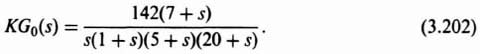
We will assume at this point that G_c1(s) = G_c2(s) = 1. Our problem is to investigate the affect of the variation of K. The transfer function of KG_c2(s)G₀(s) is given by:

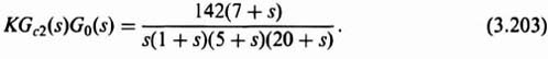
We want to consider the variation of the gain from 142 to double that amount (i.e., 248) and to one-half that amount (i.e., 71).

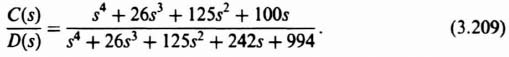
Because this control system acts as a low-pass filter, the sensitivity of H(s) with respect to K is poor. The bandwidth of this control system with K = 142 is only 3.2 rad/sec, while the sensitivity of H(s) with respect to K is expected to be greater than one at frequencies greater than 3.2 rad/sec, Figure 3.24 illustrates the unit step response of the system when K = 142 (the nominal value), K = 248, and K = 71. Table 3.1 lists the characteristics of the unit step transient responses and the characteristic equation roots of this control system which were obtained using MATLAB. Observe that variations of K from its nominal value of 142 result in considerable variation in the damping ratio and the transient responses of this control system. Figure 3.25 illustrates the root loci and the location of the closed-loop, complex-conjugate, roots for the three cases being analyzed.

Figure 3.24 Unit step response for system of Figure 3.23 with KG_c2(s)G₀(s) given by Eq. (3.203) and G_c1(s) = 1.

Table 3.1. Characteristics of the Control System Illustrated in Figure 3.23 where KG_c2(s)G₀(s) is given by Eq. (3.203), and G_c1(s) = 1

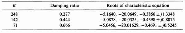
The design approach for this robust controller, G_c2(s), is to place two zeros at (or near) the desired complex, conjugate-loop, poles at −0.4398 ± j0.8875 for the nominal gain case of K = 142. Therefore,

or

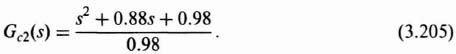
We will approxinate G_c2(s) as follows:

Therefore, the forward-path transfer function of this control system with KG₀(s) given by Eq. (3.202) and G_c2(s) given by Eq. (3.206) is:

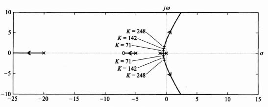
Figure 3.25 Root-locus plot for system of Figure 3.23 with KG_c2(s)G₀(s) given by Eq. (3.203) and G_c1(s) = 1.

Table 3.2 lists the damping ratio and the characteristic equation roots of this control system, obtained using MATLAB, with the forward-loop transfer function given by Eq. (3.207). Observe that the range of the damping ratios are much closer (0.548 to 0.808) than they were before the addition of the robust controller G_c2(s) and shown in Table 3.1 (where the damping previously varied from 0.277 to 0.666).

Figure 3.26 illustrates the root loci with the robust controller G_c2(s) added, and the location of the closed-loop, complex-conjugate, roots for the three cases. Observe from this root locus that by locating the two zeros of the forward-loop controller G_c2(s) near the desired characteristic equation complex- conjugate roots for K = 142, the sensitivity of this control system becomes much better.

It was shown in Section 3.2 during the discussion on the concept of liner-state-variable feedback that for the system illustrated in Figure 3.3, the zeros of C(s)/R(s) are the zeros of G(s) based on comparing Eqs. (3.17) and (3.24). Therefore, in the system we are currently analyzing in Figure 3.23, the zeros of the forward-path transfer function KG_c2(s)G₀(s) are identical to the zeros of the closed-loop transfer function. Therefore, the closed-loop zeros of G_c2(s) in Eq. (3.206) come close to canceling the effect of the complex-conjugate, closed-loop poles. Therefore, it is necessary to also add the series controller G_c1(s), as illustrated in Figure 3.23, so that G_c1(s) contains poles to cancel the zeros of s² + 0.88 + 1 of the closed-loop transfer function. Therefore, the transfer function of the forward-loop controller, G_c1(s), is given by:

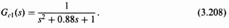
Table 3.2. Characteristics of the Control System Illustrated in Figure 3.23 with the Forward-Loop Controller G_c2(s) added and where KG_c2(s)G₀(s) is given by Eq. (3.207)

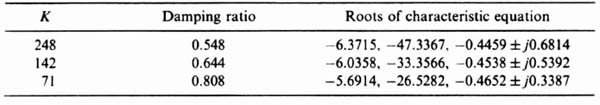
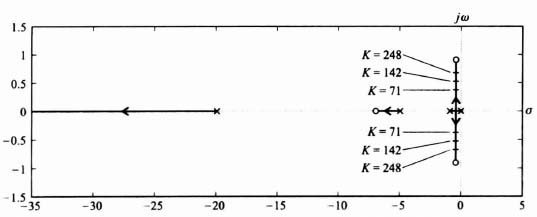
Figure 3.26 Root-locus plot for system shown in Figure 3.23 with KG_c2(s)G₀(s) given by Eq. (3.207).

The unit step response of this control system with the forward-path transfer function of the control system given by Eq. (3.207), with K = 71, 142, and 248, and with the forward-loop controller transfer function given by Eq. (3.208) is illustrated in Figure 3.27. Comparing these unit step responses with those in Figure 3.24, we conclude that this control system has been made to be much less sensitive to variations in K. For example, the maximum percent overshoot of the transient responses for the original system illustrated in Figure 3.24 ranged from 5.6% (for K = 71) to 39% (for K = 248). However, the control system designed to be robust has a transient response as illustrated in Figure 3.27 which shows that the maximum percent overshoot varies from 1.4% (for K = 71) to only 13% (for K = 248). In addition, as we pointed out before in comparing Eqs. (3.198) and (3.201), which are identical, the robustness with respect to variations in K will also provide disturbance suppression using the same control-system techniques.

Since the disturbance suppression attributes are a function of frequency, let us examine the frequency characteristics of the C(s)/D(s) transfer function. Substituting Eq. (3.203) into Eq. (3.198), we obtain the following transfer function for C(s)/D(s) for the case where the forward-loop controller G_c2(s) has a gain equal to one:

Substituting Eq. (3.207) into Eq. (3.198), we obtain the following transfer function for C(s)/D(s) for the case where the forward-loop controller G_c2(s) has the transfer function given by Eq. (3.206)

Figure 3.27 Unit step response for system of Figure 3.23 with KG_c2(s)G₀(s) given by Eq. (3.207) and G_c1(s) given by Eq. (3.208).

Figure 3.28 is a plot of the frequency response of the disturbance suppression transfer fucntion C(s)/D(s) as defined in Eqs. (3.209) and (3.210). It shows that the disturbance suppression of the control system at low frequencies is approximately the same with and without G_c2(s) in the control system. However, the addition of G_c2(s), as defined by Eq. (3.206), greatly improves the disturbance suppression attributes of the control system at high frequencies. This is consistent with our expectations.

Robust control-system design principles are being applied to many, modem, practical control systems. For example, the reader is referred to Reference 15 which presents the design for a robust control system for preventing car skidding. A complete case study for the design of a robust control system for controlling the flaps of a hydrofoil is presented in Section 7.7.

3.11. AN INTRODUCTION TO H^∞ CONTROL CONCEPTS [16, 17]

In the presentation of this book, the classical frequency-domain approach and the modern state-variable time-domain approach have been presented in parallel. It has been shown that they complement each other. Prior to the 1960s, the frequency-domain approach predominated. With the advent of the space race, the availability of practical digital computers, modern optimal control theory, and the state-variable approach in the early 1960s, the pendulum swung to the time-domain approach. The 1960s and 1970s saw an abundant amount of work performed on applying modern optimal control theory, which is presented in Chapter 6 in this book. In the early 1980s, a new technique has emerged known as H^∞ control theory which combines both the fequency- and time-domain approaches to provide a unified answer. Zames is given credit for its introduction with his paper in the IEEE Transactions on Automatic Control [16]. The H^∞ approach has dominated the trend of control-system development in the 1980s and 1990s. A complete treatment of the subject of H^∞ is complex, and beyond the scope of this book. However, we can expand the concepts of robustness (introduced in Section 3.10) and sensitivity (introduced in Chapter 1), together with the frequency and state-variable domain techniques presented in this book to introduce the basic concepts of H^∞ control theory and apply it to some simple problems. This is the objective of this and the following sections.

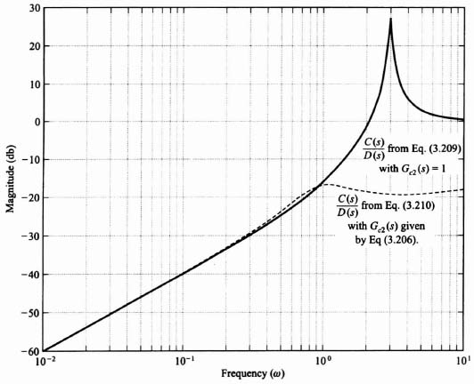
Figure 3.28 Frequency response of the disturbance suppression transfer functions defined in Eqs. (3.209) and (3.210).

A. Sensitivity of Control Systems Containing Disturbances and Measurement Noise

Let us extend our understanding of sensitivity developed in Chapter 1 to the control system illustrated in Figure 3.29 which contains a disturbance U(s) and feedback sensor measurement noise N(s). Although noise is a stochastic process, we will assume in this analysis that it can be represented as a deterministic process. This initial analysis will focus on the single-input single-output (SISO) system shown in Figure 3.29 which contains a disturbance U(s) and feedback sensor measurement noise N(s). We will then discuss the extension of these results to multiple-input multiple-output (MIMO) systems.

Using Mason's theorem, we can write the following relationship for the output C(s) by inspection of Figure 3.29:

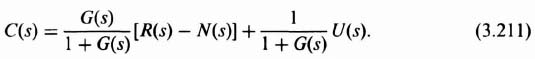
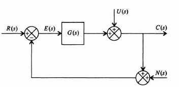
Figure 3.29 Control system containing a disturbance U(s) and sensor measurement observation noise N(s).

We can also use Mason's theorem to write the following relationship for the control-system error E(s) by inspection of Figure 3.29:

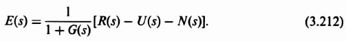
From the analysis in Section 1.7 on sensitivity, we know that the sensitivity of the transfer function C(s)/R(s) to changes in G(s) for the control system shown in Figure 3.29 is given by the following expression:

It is interesting to observe that this sensitivity is also the transfer function from U(s) to −E(s):

In the MIMO case, the sensitivity function in Eq. (3.213) is modified so that G(s) becomes the matrix of transfer functions between the inputs and the outputs, and the value of I is replaced with the identity matrix.

The transfer function C(s)/R(s) of the control system shown in Figure 3.29 is given by the following:

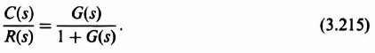
This expression is also known as the complementary sensitivity function which is defined as follows:

It is very important to recognize that the sum of the sensitivity function given by Eq. (3.213), and the complementary sensitivity function given by Eq. (3.216) equals one:

We can express the error function E(s) in Eq. (3.212) in terms of the sensitivity function. Let us assume that the feedback sensor measurement noise is zero. Therefore, substituting Eq. (3.213) into Eq. (3.212), we obtain the following:

Equation (3.218) is a very important relationship because it states that we should make the sensitivity function S small to make the control system error E(s) small. In addition, we know that since Eq. (3.213) represents the sensitivity function as well as the transfer function between U(s) and −E(s) [see Eq. (3.214)], we want the sensitivity function S(s) to be as small as possible for both disturbance rejection and for making the control-system error small.

The conclusion of this analysis is that we want to make S(s) as small as possible. However, is this possible over the entire range of frequencies? Let us analyze Eq. (3.213) to determine if this is feasible. Since G(s) approaches zero as s approaches infinity in practical systems, then

The result of Eq. (3.213) is that we can only make the sensitivity function S(s) small over low and mid-range frequencies, but not at high frequencies.

Ideally, what would we like to make the complementary sensitivity function? Analyzing Eq. (3.217), we would like to make the complementary sensitivity function T(s) equal to one because that would then result in the sensitivity function S(s) being equal to zero. However, we know from Eq. (3.216) that T(s) approaches zero as G(s) approaches infinity. Therefore, we can design the complementary sensitivity function T(s) to approximate one at low and mid-range frequencies, but not at high frequencies. Figure 3.30 illustrates the representative frequency responses of the sensitivity function S(s) and the complementary sensitivity function T(s).

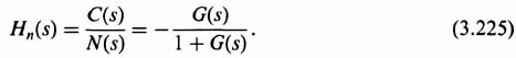
The transfer function relating the sensor measurement noise N(s) to the output C(s) can be obtained from Eq. (3.211) by setting R(s) = U(s) = 0:

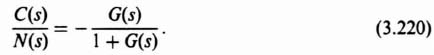
Observe that Eq. (3.220) is the negative of the complementary sensitivity function T(s) defined in Eq. (3.216). Therefore,

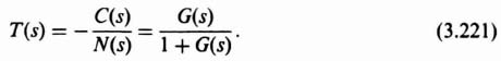
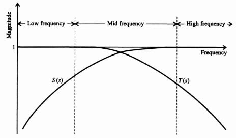
Figure 3.30 Representative sensitivity and complementary sensitivity frequency responses.

This results in a problem to the control-system engineer because we want the transfer function C(s)/N(s) to be as small as possible, but the desirable T(s) is large at low and mid-range frequencies as illustrated in Figure 3.30. Equation (3.217) showed that we would want to make T(s) = 1 ideally in order to drive the sensitivity function S(s) = 0. Therefore, the control-system engineer must make a tradeoff here between allowable feedback sensor measurement noise and the complementary sensitivity function (which also affects the sensitivity function [see Eq. (3.217)]. The basic tradeoff is to determine allowable noise and permissible sensitivity.

B. Desirable Control-System Transfer-Function Characteristics

From Figure 3.29 and Eq. (3.211), we can state the relationship between the reference input R(s), the disturbance U(s), and the feedback sensor measurement noise N(s) with the output C(s) as follows:

where

In terms of the error function E(s), as defined in Eq. (3.212), we define E(s) as follows:

It is interesting to examine the effect of the feedback sensor noise on the control system. To do this, let us assume that all the other external inputs are zero:

Let us assume that n(t) has a Fourier transform although, in practice, noise usually does not have a Fourier transform. Using Parseval's theorem, we can determine the integral-squared error (ISE):

By focusing on the square of the error, the ISE penalizes both positive and negative values of the error. The function |N(jω)|² is defined as the energy density spectrum of ω.

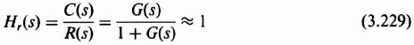
Let us try to define the desirable frequency characteristics from a practical viewpoint for H_r(jω), H_u(jω), and H_n(jω). The reference input R(s) and the disturbance U(s) are usually low-frequency signals. Therefore, it is desired to have H_r(jω) 1 and H_u(jω) 0 at low frequencies. In practice, H_r(jω) 0 and H_u(jω) and H_n(jω) 1 at high frequencies. In practice, we try to make H_r(jω) 1, and H_u(jω) and H_n(jω) 0 over the frequency range from 0 to the gain crossover frequency ω_c. These are ideals and, in practice, we can only approximate these. For example, Figure I1.7-3 shows the closed-loop frequency response of Figure I1.7-1. This closed-loop frequency response corresponds to H_r(s) for the system shown in Figure I1.7-1.

In practice, G(s) is much greater than one at low frequencies. Therefore, Eq. (3.223) reduces to

and Eqs. (3.224) and (3.225) reduce to

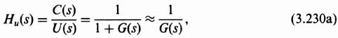
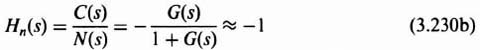
at low frequencies. Therefore, a high loop gain is very desirable for frequencies in the passband (defined as frequencies between 0 and ω_c) because it then approximates H_r(jω) 1 and H_u(jω) is very small. However, the sensor measurement observation noise remains a problem because H_n(s) is approximately −1. The control engineer has two choices regarding N(s): (a) Design the sensor so that its measurement noise is very small; (b) tradeoff how high the loop gain is designed so that it minimizes the effect of the disturbance input U(s), but the loop gain should not be too high so that the effect of the noise is tolerable.

C. Extension of Sensitivity and Complementary Sensitivity Concepts to Multivariable Control Systems

Many modern control systems contain several inputs and outputs. Therefore, it is important to extend our understanding of sensitivity and complementary sensitivity to multiple-input multiple-output (MIMO) control systems.

Figure 3.31 illustrates the block diagram of a MIMO control system where r(t) and c(t) are vectors, and D(s) and G(s) are matrices. The dimensions of D(s) are n × i, and the dimensions of G(s) are i × n, where n = dim[C(s)] and i = dim[m(s)]. By analogy to Eq. (3.213) for the SISO control system, the sensitivity function for the MIMO control system is given by:

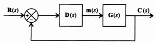
Figure 3.31 Block diagram of a MIMO control system.

By analogy to Eq. (3.216) for the SISO control system, the complementary sensitivity function for the MIMO control system is given by

The sensitivity and complementary sensitivity functions are both n × n matrices. By analogy to Eq. (3.217) for the SISO case, the sum of the sensitivity and complementary functions for the MIMO case is given by

where I represents the identity matrix.

D. Example for Finding S(s) and T(s) for a MIMO Control System

The open-loop transfer function matrix for a two-input, two-output control system to be analyzed is given by

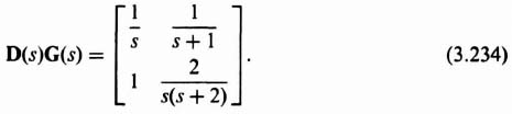
Let us determine the sensitivity and the complementary sensitivity functions.

The sensitivity function for this MIMO control system is obtained from Eq. (3.231) as follows:

Therefore,

The complementary sensitivity function T(s) can be found from

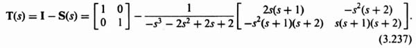
Simplifying this expression, we obtain

3.12. FOUNDATIONS OF H^∞ CONTROL THEORY

Based on the preceding results, the concepts of modern H^∞ control theory will be presented. The very basic problem that H^∞ as presented by Zames in Reference 16 focuses on is sensitivity reduction of feedback control systems as an optimization problem, and it is separated from the problem of stabilization. The technique is concerned with the effects of feedback on uncertainty, where the uncertainty may be in the form of an additive disturbance U(s) as illustrated in Figure 3.29. H^∞ control theory approaches the problem from the point of view of classical sensitivity theory, which has been presented in Chapter 1 and subsections 3.11A–3.11D, with the difference that feedback will not only reduce but also optimize sensitivity in an appropriate sense.

H^∞ control theory is a complex subject. The purpose of presenting it in this book, in a clear and cohesive manner, is to introduce it and motivate the reader with an interest in this field to review fome of the recent papers which have been written on this subject [18–21]. In its basic form H^∞ control theory attempts to minimize the supremum function over the entire frequency range

where S(jω) is the sensitivity function and W(jω) is a weighting function. We can view the magnitude of the product S(jω)W(jω) as the magnitude of the weighted sensitivity. The weighting function emphasizes that low sensitivity is more important at low frequencies than higher frequencies. Therefore, by emphasizing the minimization of the magnitude of the product, the result is that the weighting function is greatest at those frequencies where the sensitivity is the smallest-namely at low frequencies.

The general solution to Eq. (3.239), obtained from function analysis, has the following general form [21]:

where k is a constant and B(s) is known as the Blaschke product. For the problem being considered in this book where the process G(s) is stable (e.g., all of its poles are in the left-half of the s-plane and are of minimum phase), then B(s) = 1 and the constant k is any desirable, small, real number. Therefore, Eq. (3.240) states that we want to make the weighting function large for those low frequencies where we want to make the sensitivity small. Conversely, we want to make the weighting function small for those high frequencies where the sensitivity is large.

Let us examine in detail the result when G(s) has all its poles in the left-half of the s-plane, and B(s) = 1. Therefore,

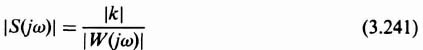
which implies that the shape of the magnitude of the sensitivity curve is the inverse of the weighting function. Therefore, the shape of the optimum |S(jω)| is independent of the process G(s), and only depends on the magnitudes of the constant k and the weighting function W(jω).

A. Application of the Theory to an Example

Let us try to pull all the concepts presented in this section together by giving an example. We will consider a simple SISO control system, and determine its sensitivity function, S, complementary sensitivity function, T, and the weighting function, W. We will also assume that the constant k in Eq. (3.240) is equal to one.

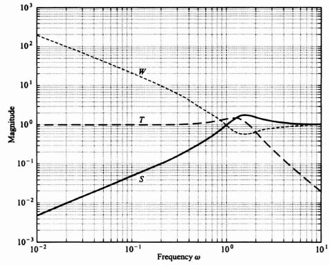
For the illustrative example, let us consider a unity-feedback control system whose forward transfer function G(s) is given by

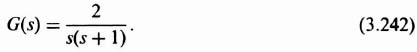
Substituting Eq. (3.242) into Eqs. (3.213), (3.216), and (3.241), we can calculate the sensitivity S, the complementary sensitivity T, and the weighting function W, respectively. The result is shown in Figure 3.32. The result agrees with the theoretical results expected from the presentation of this section. The sensitivity S is very small at low frequencies, and approaches one at very high frequencies. The weighting function W is the inverse of the sensitivity function, and is very large at low frequencies and also approaches one at very high frequencies. The complementary sensitivity function equals one minus the sensitivity function (see Eq. (3.217)), and equals one at very low frequencies and is very small at very high frequencies.

B. The H^∞ Process for the General SISO Case

Let us assume that in the general SISO case, the process G(s) has poles and zeros in the right half-plane. For this general case, the H^∞ process would proceed in the following step-by-step manner:

1. The weighting function W(s) would be selected which would have the following characteristics:

• It must have no zeros in the right half-plane.

  

  Figure 3.32 S, T and W for a unity-feedback system with G(s) = 2/s(s + 1).

• It must contain any poles that G(s) has on the jω axis.
• It must not contain jω poles at zeros of G(s).

2. Determine the Blaschke product B(s) from knowledge of the poles of G(s). If G(s) has no poles in the right half-plane as illustrated in the preceding example in subsection 3.11A, B(s) = 1. Let us next consider the general case where G(s) has poles in the right half-plane. Therefore, from Eq. (3.240),

where P_n are poles of G(s) in the right half-plane.

3. S(P_n) has to satisfy the following interpolation conditions for simple poles and zeros of G(s) in the right half-plane:

• S equals zero at right-half poles, and one at right-half zeros.
• T is one at right-half poles and zero at right-half zeros.

This can be shown as follows. Let us consider the control system in Figure 3.33. The sensitivity of C(s)/R(s) to D(s)G(s) is given by

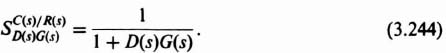
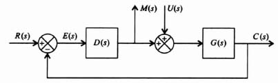
Figure 3.33 General SISO control system containing a reference input, R(s), and a disturbance signal, U(s).

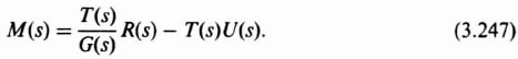
The complementary sensitivity function is given by

The transfer functions between the inputs R(s) and U(s), and the outputs M(s) and C(s) are given as follows:

In terms of T(s) given by Eq. (3.245), Eq. (3.246) can be written as

Therefore,

Equation (3.248) can be reduced to the following:

In terms of T(s) and S(s), Eq. (3.249) can be rewritten as follows:

Analysis of Eq. (3.247) reveals the following:

• If T(s)/G(s) is to be stable, then T(s) must cancel the right-half zero(s) of G(s).

Analysis of Eq. (3.250) reveals the following:

• If G(s)S(s) is to be stable, then S(s) must cancel the pole(s) in the right-half plane of G(s).

These two very important interpolation conditions imply that for simple zeros and poles which are in the right half-plane, S(s) equals one at the right-half-plane zeros, and S(s) equals zero at the right-half plane poles. Similarly, T(s) equals zero at the right-half plane zeros, and T(s) equals one at the right-half-plane poles in accordance with Eq. (3.217).

4. Form the Blaschke product. Returning to Eq. (3.243), and recognizing that S(P_n) must satisfy these interpolation conditions, what should B(P_n) and W(P_n) be? Let us assume that G(s) has poles in the right half of the s-plane, and let P_n, n = 1, 2, …, N, be poles of G(s). Therefore, Eq. (3.243) must be satisfied for the interpolation conditions. Because the weighting function W(s) has no poles in the right half-plane, it cannot equal infinity. Therefore, it is necessary to have the Blaschke product B(s) contain the zeros of S(p_n):B(p_n) = 0, n = 1, 2, 3…, N. This means that the Blaschke product accounts for these zeros as follows:

where

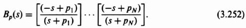
We can find B'(s) from the interpolation conditions previously shown. For example, let us assume that these zeros in the right half-plane which force S(s) to equal one at these zeros are Z₁, Z₂, Z₃,…, Z_M. From Eqs. (3.243) and (3.251),

This equation can be simplified to

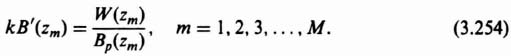
Equation (3.254) represents M equations which must be solved. It can be shown that if M = 1, then B'(s) = 1. If M is greater than one, then

where c_i, are complex values with the positive real parts chosen, together with the value of k, to satisfy Eq. (3.254).

5. Solve for S(s). Having solved B'(s), the optimal sensitivity S(s) is then calculated from the following equation which is obtained by substituting Eq. (3.251) into Eq. (3.240):

The resulting S(s) is stable because B'(s) and B_p(s) are stable, and since W(s) has no poles in the right half-plane. Because |B(jω)| = 1

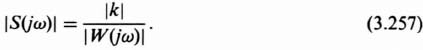
Therefore, this equation shows that the magnitude of the sensitivity curve is the inverse of the magnitude of the weighting function curve. It is also interesting to observe that the optimal |S(jω) is independent explicitly of G(s). However, G(s) does effect the value of k.

C. An Example of the SISO Case Containing a Pole in the Right Half-Plane

Consider the control system illustrated in Figure 3.33 where

and the weighting function W(s), shown in Figure 3.34, is given by

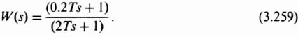
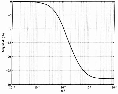
Figure 3.34 Weighting function W(s).

This weighting function gives more weight to low frequencies (up to the bandwidth 1/2T) than high frequencies. From Eq. (3.252), the right-half pole of G(s) at s = 3 results in B_p(s) given by

Because D(s)G(s) has only one zero at s = 2 in the right half-plane of the s-plane, then B'(s) = 1. Therefore, from Eq. (3.254), we can find k as follows:

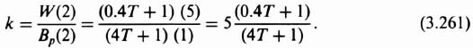
Substituting k from Eq. (3.261), B_p(s) from Eq. (3.260), and W(s) from Eq. (3.259) into Eq. (3.256) we can solve for the optimal sensitivity S(s):

We can obtain the absolute value of the optimal sensitivity function from Eq. (3.257) as follows:

Figure 3.35 illustrates the absolute value of the sensitivity function obtained from Eq. (3.263) for values of T = 0.2, 2, and 20. It is concluded from this curve that the sensitivity is smaller (better) at low frequencies if the bandwidth is not too high (or T is not too small).

3.13. LINEAR ALGEBRAIC ASPECTS OF CONTROL-SYSTEM DESIGN COMPUTATIONS [22–25]

The fundamental problems of linear control-system theory were reconsidered at the end of the 1960s and the beginning of the 1970s. The algebraic characteristics of the control-system problems were reestablished and have resulted in a better understanding of the foundations of linear control-system theory.

This section focuses on the interplay between some recent results and methodologies in numerical linear algebra and their application to problems arising in control systems. Let us reconsider the phase-variable canonical form representation of a control system:

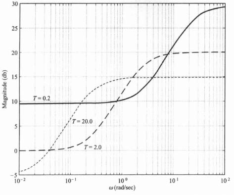
Figure 3.35 Optimal sensitivity frequency characteristic as a function of T.

We can represent this canonical form representation in terms of its frequency response by using Eqs. (3.10) and (3.18):

The problem of computing C(s)/R(s), or C(jω)/R(jω), from knowledge of K, P, b, L, and h, efficiently is a practical problem of great interest. Reference 23 presents an efficient and generally applicable algorithm to solve this problem. The approach recommended performs an initial reduction of P to upper Hessenberg form H, rather than solving the linear equation (with dense, unstructured P) (jωI – P)X = b, which would require O(n³) operations for each successive value of ω. The orthogonal matrices used to effect the Hessenberg form of P are incorporated into b and L giving and . Therefore, as ω varies, the coefficient matrix in the linear equation remains in upper Hessenberg form. The advantage is that X can be determined in O(n²) operations rather than O(n³) as before, which is a very significant saving. In addition, this methodology is numerically very stable and has the advantage of being independent of the eigenstructure (possibly ill-conditioned) of P.

This methodology can be extended to state-variable models in implicit form. For example, let us replace Eq. (3.264) by

Therefore, Eq. (3.266) can be replaced with the following:

We can use the initial triangular/Hessenberg reduction to again reduce the problem to one of updating the diagonal of a Hessenberg matrix and, therefore, an O(n²) linear equation problem. [24].

3.14. ILLUSTRATIVE PROBLEMS AND SOLUTIONS

This section provides a set of illustrative problems and their solutions to supplement the material presented in Chapter 3.

1. I3.1. The state and output equations of a second-order control system are given by the following:

   

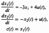
   where x₁(t) and x₂(t) represent the system states, c(t) is the system's output, and u(t) represents its input.

   1. Determine whether the system is controllable.
   2. Determine whether the system is observable.

   SOLUTION:

   1. From Eq. (3.65) controllability can be determined for this second-order system from:

      

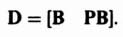
      The phase variable canonical form of the state and output equations can be written as:

      

      Therefore the companion matrix, P is given by

      

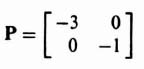
      and the input vector, B, is given by

      

      and the output matrix is given by:

      

      Therefore, the matrix D is given by:

      

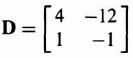
      and the system is controllable.

   2. Observability can be determined for this second-order control system from Eg. (3.75) where

      

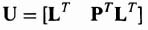
      Therefore, the matrix U is given by:

      

      So, the system is unobservable because U is singular.

2. I3.2. Synthesize a system using linear-state-variable feedback that has a closed-loop transfer function given by

   

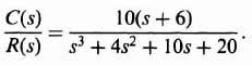
   Assume that the proces to be controlled has a transfer function given by

   

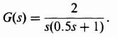
   In your solution, show the following:

   1. Synthesis of the linear-state-variable-feedback system.
   2. Identification of any compensation network needed to satisfy the synthesis. What kind of network is it?
   3. Check of the stability of the resulting system synthesized using the root-locus method.

   SOLUTION:

   1. 

      Figure I3.2(i)

      

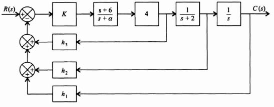
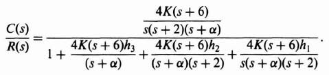
      This equation can be reduced to the following:

      

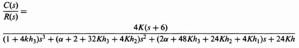
      Comparing the coefficients of this equation for the synthesized linear-state-variable-feedback system and that of the desired closed-loop transfer function given by

      

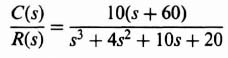
      we obtain the following five simultaneous equations to be solved:

      

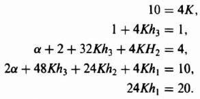
      Therefore, we obtain the following results:

      

   2. The compensation network is given by

      

      which is a phase-lag network.

   3. The root locus is drawn from the following transfer function:

      

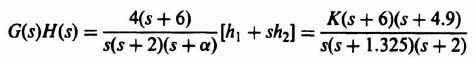
      The following root-locus diagram shows that this control system is stable for 0 < K < ∞:

      

      Figure I3.2(ii)

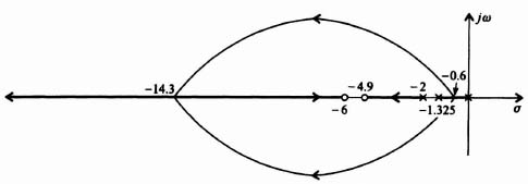
3. I3.3. Design a third-order controller whose three roots are located at the following locations in the s-plane: −1; −1; −12. The transfer function of the system to be controlled is given by

   

   Determine the controller gain matrix, K.

   SOLUT1ON: The desired location of the controller roots are located at:

   

   We need to determine the companion matrix, P, and the input gain vector, b, so that we can solve for the controller gain matrix, K from Eq. (3.167). The states of this third-order control system are defined as follows:

   Let x₁ = c(t); x₂ = c(t); . Therefore, the state equations are given by:

   

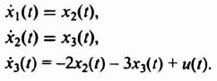
   The state equations in their vector and matrix format are given by:

   

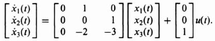
   Therefore, the companion matrix, P, is given by:

   

   The controller gain K can be determined from Eq. (3.167) as follows:

   

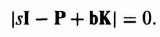
   Substituting into Eq. (3.167), we obtain the following:

   

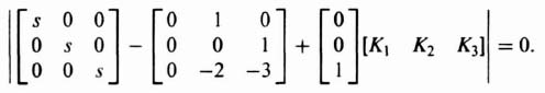
   This can be simpified to

   

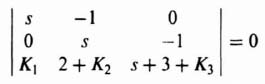
   which can be reduced to the following:

   

   Setting coefficients of Eqs. (I3.3-1) and (I3.3-2) equal to each other, we obtain the following:

   

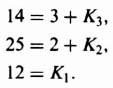
   Therefore, we solve these three equations and find that:

   

   Therefore, the controller gain matrix, K, is given by:

   

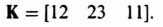
4. I3.4. Design a third-order estimator whose three roots are located at the following locations in the s-plane: −3.5; −3.5; −15. The transfer function of the process is given by

   

   Determine the estimator gain vector M.

   SOLUTION: The desired location of the estimator roots is at:

   

   We need to determine the companion matrix, P, the input gain vector, b, and the output matrix, L, so that we can determine the estimator gain factors in the M matrix from Eq. (3.131). The states of this third-order control system are defined as follows:

   Let ). Therefore, the state equations are given by:

   

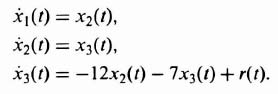
   The state equations in their vector and matrix form are given by:

   

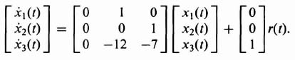
   Therefore, the companion matrix, P and the input vector, b, are

   

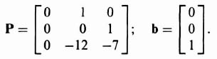
   The output equation is given by:

   

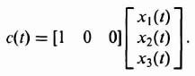
   Therefore, the output matrix is given by

   

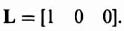
   The M matrix can be determined from Eq. (3.131) as follows:

   

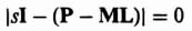
   Substituting into Eq. (3.131), we obtain the following:

   

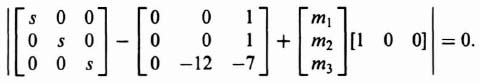
   This can be simplified to

   

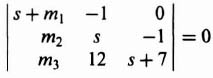
   which can be reduced to the following:

   

   Setting like coefficients of Eqs. (I3.4-1) and (I3.4-2), equal to each other, we obtain the following:

   

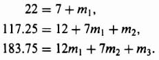
   Therefore, we solve these equations and find that:

   

   Therefore, the M vector is given by:

   

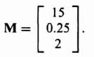
5. I3.5. Repeat the problem solved in Section 3.6 using Ackermann's Formula for a process transfer function given by

   

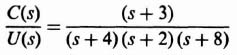
   and the control system's signal flow graph is given by:

   

   Figure I3.5(i)

   1. Determine the state equations for the process.
   2. Determine the controllability matrix for this original system.
   3. Transform the original system to the phase variable form, and determine the state and output equations.
   4. Determine the controllability matrix for the phase variable form.
   5. Determine the transformation matrix A.
   6. Design a contoller assuming that the dominant pair of complex-conjugate roots has a damping ratio of 0.707, and it results in a settling time of 4 sec. Select the third pole at the location of the zero of the process to be controlled. What is the resulting characteristic equation of the desired closed-loop control system?
   7. Determine the state and ouput equations for the phase-variable form with linear-state-variable-feedback.
   8. What is the resulting characteristic equation for the set of equations found in part (g)?
   9. Determine the linear-state-variable-feedback constants for the control system in phase-variable form.
   10. Transform the linear-state-variable-feedback constants back to the original system using the transformation matrix A.
   11. Draw the resulting closed-loop control system with linear-state-variable-feedback.

   SOLUTION:

   1. 

   2. 

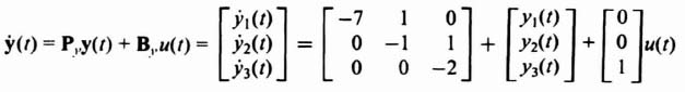
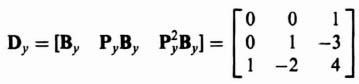
      The value of the determinant of D_y is −1, it's nonsingular, and the original control system is controllable as expected from inspection of the signal-flow graph.

   3. From the given signal-flow graph:

      

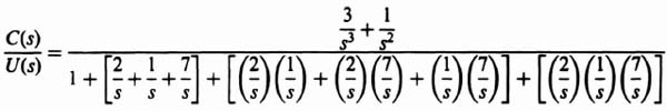
      This transfer function can be reduced to the following:

      

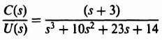
      Defining , we obtain

      

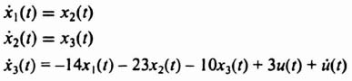
      Therefore, the state and output equations in matrix vector form of the phase variable control system are given by:

      

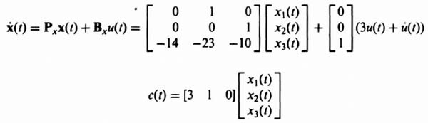
   4. The resulting controllability matrix for the phase variable form can be obtained from

      

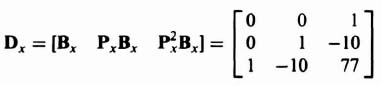
      Note that the determinant of D_x is −1 indicating that the determinant is nonsingular, and the phase variable form is also controllable, as expected.

   5. The transformation matrix, defined in Eq. (3.85) is

      

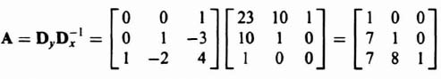
   6. A second-order control system having a damping ratio of 0.707 with a settling time of 4 seconds results in a ω_n = 1.414 [see Eq. (5.41)^‡]. Therefore, the following second-order control system can meet the design specifications:

      

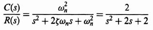
      With third pole selected at s = 3, which also cancels the zero at s = −3, the characteristic equation of the desired closed-loop system is given by:

      

   7. The state and output equations for the phase-variable form with linear-state-variable-feedback can be obtained from Eqs. (3.8) and (3.10) as follows:

      

      The state equation reduces to the following:

      

   8. The resulting characteristic equation can be obtained from Eqs. (3.10) and (3.19):

      

      Therefore,

      

      The resulting characteristic equation is given by:

      

   9. Comparing this characteristic equation (see part h) with the characteristic equation of the desired closed-loop system (see part f), results in the following:

      

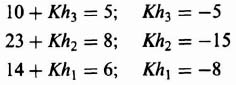
      Therefore,

      

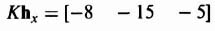
   10. We will now transform Kh_x back to the original system using Eq. (3.94) as follows:

       

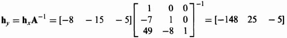
   11. The resulting closed-loop control system with linear-state-variable-feedback is the following:

       

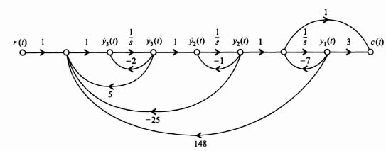
       Figure I3.5(ii) Resulting closed-loop control system wth linear-state-variable-feedback designed using Ackermann's formula.

6. I3.6. Design a combined compensator of a regulator containing a controller and estimator for the system illustrated in Figure I3.6(i).

   

   Figure I3.6(i)

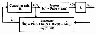
   Assume that the transfer function of the process is given by

   

   Assume that the design specification of the controller is that it is critically damped with ω_n = 3 rad/sec, and that the estimator is also critically damped with ω_n = 30 rad/sec.

   1. Find the controller's gain coefficients' matrix.
   2. Find the estimator's coefficients' vector.
   3. Determine the transfer function of the compensator for the combined controller and estimator, U(s)/C(s).
   4. Sketch the root locus of the compensated system. From your sketch, is the system unstable, stable, or conditionally stable?

   SOLUTION:

   1. The desired location of the controller roots is at:

      

      We need to determine the companion matrix, P, and the input gain vector, b, so that we can solve for the controller gain matrix, K, from Eq. (3.167). The states of this second-order control system are defined as follows:

      Let 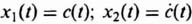. Therefore, the state equations are given by:

      

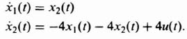
      The state and output equations in their vector and matrix format are given by:

      

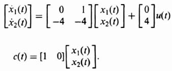
      Therefore, the companion matrix, P, the input vector, b, and the output matrix, L are given by:

      

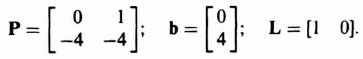
      The controller gain K can be determined from Eq. (3.167) as follows:

      

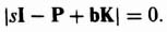
      Substituting into Eq. (3.167), we obtain the following:

      

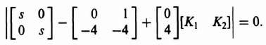
      This equation can be simplified to

      

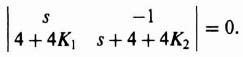
      which can be reduced to the following:

      

      Setting like coefficients of Eqs. (I3.6-1) and (I3.6-2) equal to each other, we obtain the following:

      

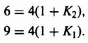
      Therefore, we solve these two equations and find that:

      

      Therefore, the controller gain matrix, K, is given by:

      

   2. The desired location of the estimator roots is at:

      

      The M matrix can be determined from Eq. (3.131) as follows:

      

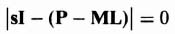
      Substituting into Eq. (3.131), we obtain the following:

      

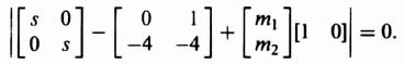
      This can be simplified to

      

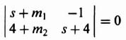
      which can be reduced to the following:

      

      Setting like coefficients of Eqs. (I3.6-3) and (I3.6-4) equal to each other, we obtain the following:

      

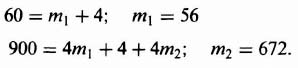
      Therefore, the M vector is given by:

      

   3. The transfer function of the compensator, U(s)/C(s) can be determined from Eq. (3.162):

      

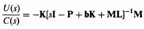
      Substituting values for K, P, B, and L found in part (a), and M found in part (b), we obtain the following:

      

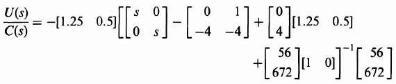
      which reduces to

      

      Further reduction reduces this equation to the following:

      

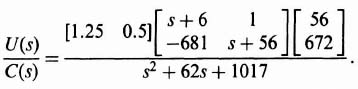
      This equation reduces the following expression for the transfer function of the compensator for the combined controller and estimator, U(s)/(C(s):

      

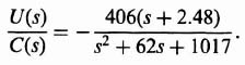
      This is a phase-lead network having the zero at s = −2.48.

   4. The root locus for the compensated system is plotted from the following expression:

      

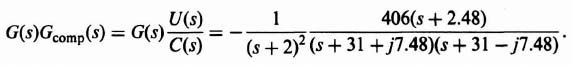
      The root locus shown in Figure I3.6(ii) shows that this is a conditionally stable system that is stable for < K < 61, 102. Observe that the root locus goes through the roots chosen for the controller roots (s = −3, −3) and estimator roots (s = −30, −30)

      

      Figure I3.6(ii)

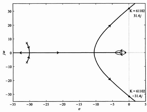
7. I3.7. The system of Problem I3.6 is modified to respond to a reference input, r(t), as shown in the following block diagram:

   

   Figure I3.7

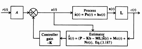
   Assume that the process, combined compensator containing a controller and an estimator, and the specifications for the controller and estimator are exactly the same as in Problem I3.6. Assuming that A = 4, determine the requirement on M so that the state-estimation error is independent of the reference input, r(t).

   SOLUTION: We can determine the requirement on N so that the state-estimation error is independent of the reference input, r(t), from Eq. (3.193):

   

   From Problem I3.6, we know that the input vector, b, is given by

   

   Substituting b and A = 4 into Eq. (3.193), we obtain the following:

   

   Therefore, N is given by

   

8. I3.8. We wish to design a robust control system containing a two-degrees-of-freedom series controller G_c1(s) and a forward-loop-controller G_c2(s) which is illustrated as follows:

   

   Figure I3.8(i)

   The transfer function KG₀(s) is

   

   The gain of this transfer function can vary significantly, and the value of 150 is only the nominal amount. During its operation, the gain has been known to go as low as 75 and as high as 300. The objective of the control-system engineer is to design the robust control system shown so that the effect of this wide gain variation is minimized on the control system's transient response.

   1. Determine the control system's transient response to a unit step input for K = 75, 150, and 300, assuming that G_c1(s) = G_c2(s) = 1.
   2. Draw the root locus for the conditions defined in part (a).
   3. From the root locus drawn in part (b), determine the location of the roots for the closed loop system for gains of 75, 150, and 300, and the damping and overshoot, for the dominant set of complex-conjugate roots, for the three sets of gains being considered.
   4. Design the robust controller G_c2(s).
   5. Determine the transfer function KG_c2(s)G₀(s).
   6. Plot the root locus for the transfer function determined in part (e), and determine the damping, overshoot, and the roots of the characteristic equations for gains of 75, 150, and 300.
   7. Determine the design of the forward-loop controller G_c1(s) in this two-degrees-of-freedom control system.
   8. With G_c1(s), as determined in part (g) added to this control system, determine the transient response of this control system to a unit step input for K = 75, 150, and 300.
   9. What conclusions can you reach from the resulting transient responses found in parts (a) and (h)?

   SOLUTION:

   1. Figure I3.8(ii) illustrates the unit step responses for this control system for K = 75, 150, and 300 which was obtained using MATLAB. Observe from this figure that the peak overshoot varies from 27.3% for K = 75, to 69.3% for K = 150, and 76.3% for K = 300.
   2. The root locus obtained from MATLAB is shown in Figure I3.8(iii).
   3. Table I3.8(i) lists the damping, overshoot, and the characteristic equation roots for the dominant set of complex-conjugate roots of this control system.

      Observe from this table the considerable variation in the damping ratio and the maximum percent overshoot (based on the dominant complex-conjugate roots) for the three cases being analyzed.

   4. The robust controller has the following pair of complex-conjugate zeros to cancel the poles of the system where K = 150:

      

      Figure I3.8(ii) Unit step response of KG(s) = K(s + 12)/s(s + 2)(s + 8)(s + 25).

      

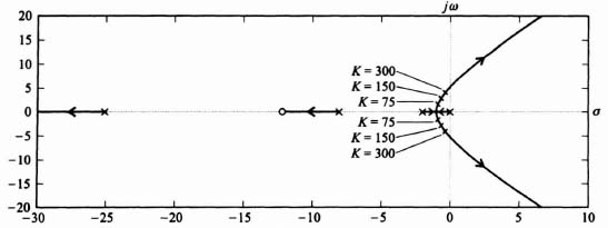
      Figure I3.8(iii) Root-locus plot for system shown in Figure I3.8(i) for KG₀(s) as defined in Eq. (I3.8-1) and G_c1(s) = G_c2(s) = 1.

      Table I3.8(i)

      

      

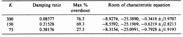
      Figure I3.8(iv) Root-locus plot for system shown in Figure I3.8(i) with KG_c2(s)G₀(s) given by Eq. (I3.8-3).

      

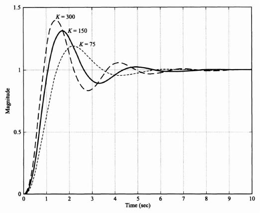
      Figure I3.8(v) Unit step response of KG(s) = K(s + 12)/s(s + 2)(s + 8)(s + 25) with robust control.

      Table I3.8(ii)

      

      

   5. 

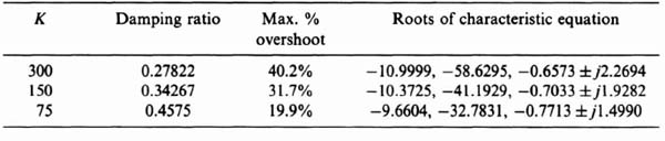
   6. The root locus, which was obtained using MATLAB, is illustrated in Figure I3.8(iv). From this root locus, the damping ratio, maximum percent overshoot, and roots of the characteristic equation are shown in Table I3.8(ii):
   7. The design of the forward-loop controller G_c1(s) is the reciprocal of the robust controller G_c2(s):

      

   8. The resulting transient response of this control system to a unit step input for K = 75, 150, and 300 is illustrated in Figure I3.8(v).
   9. The resulting transient response illustrated in Figure I3.8(v) shows that the maximum percent overshoots with the robust control design have been greatly reduced from those illustrated in Figure I3.8(ii). The new robust control-system design truly exhibits admirable robust control features. Table I3.8(iii) compares the transient response with and without robust control:

      Table I3.8(iii)

      

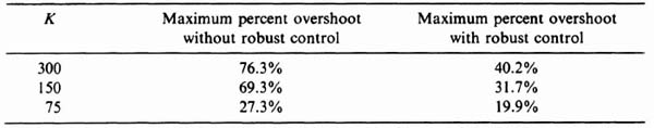
      In addition to the reduction in the maximum percent overshoots, observe that the range of the maximum percent overshoots is reduced from 76.3%/27.3% = 2.79 without robust control to 40.2/19.9% = 2.02. That is a very significant reduction which robust control makes possible. Therefore, the robust system is much less sensitive to variations in K. In addition, the robustness with respect to variations in K will also provide disturbance suppression to D(s).

9. I3.9. The optimal sensitivity function for the control system illustrated in Figure I8.9(i) is to be determined in the H^∞ sense.

   

   Figure I3.9(i)

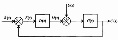
   The transfer function of the process G(s) is given by

   

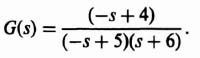
   The weighting function W(s) is given by

   

   1. Determine the value of B_p(s).
   2. Determine the value of the constant k.
   3. Determine the value of the optimal sensitivity function S(s).
   4. Determine the absolute value of the optimal sensitivity function and plot the results for T = 0.2, 2, and 20 sec.
   5. What conclusions can you reach from these curves?

   SOLUTION:

   1. From Eq. (3.252), the right-half pole of G(s) at s = 5 results in

      

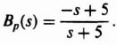
   2. Because G(s) has only one zero in the right half-plane of the s-plane, then B'(s) = 1. Therefore, from Eq. (3.254), we can find k as follows:

      

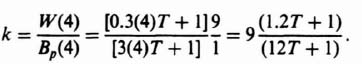
   3. Substituting into Eq. (3.256) for k, B'(s), B_p(s), and W(s), we obtain the following:

      

   4. The absolute value of the optimal sensitivity function can be obtained from Eq. (3.257) as follows:

      

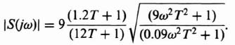
      The absolute value of the sensitivity function is plotted in Figure I3.9(ii) for the following values of T: 0.2, 2, and 20.

      

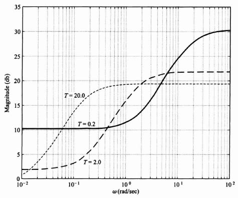
      Figure I3.9(ii) Optimal sensitivity frequency characteristic as a function of T.

   5. It is concluded from these curves that the sensitivity is smaller (better) at low frequencies if the bandwidth is not too high (or T is not too small).

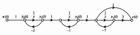
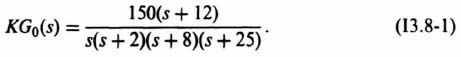
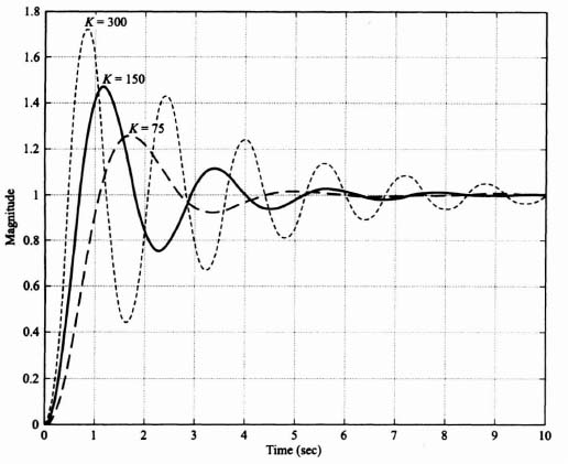
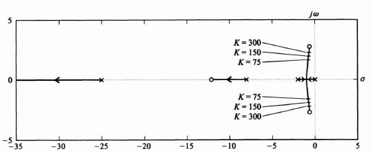
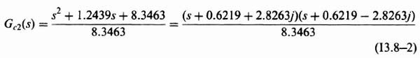
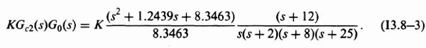
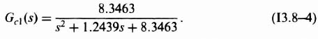
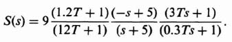
PROBLEMS

1. 3.1. The control system illustrated in Figure P3.1(i) contains linear-state-variable-feedback elements h, and h₂.
   1. Determine the gain K and the linear-state-variable-feedback constants h₁ and h₂ so that the resulting control system represents a zero steady-state step error system and its characteristic equation contains roots at −2 + j, −2 − j, and −8.

      

      Figure P3.1(i)

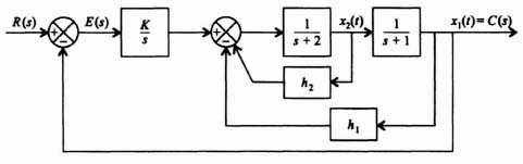
   2. The same performance can be obtained as in part (a) if we implement a series controller, G_c(s), instead of using linear-state-variable-feedback as illustrated in the configuration shown in Figure P3.1(ii).

      

      Figure P3.1(ii)

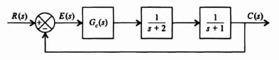
      Determine the transfer function of G_c(s) in terms of K, h₁, and h₂ obtained in part (a) and the other system parameters provided.

2. 3.2. A control system containing a controller and a process are illustrated in the block diagram in Figure P3.2(i).

   

   Figure P3.2(i)

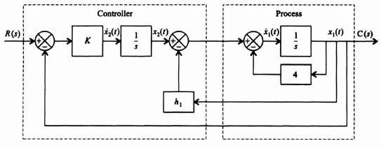
   1. Determine the state equations of this control system.
   2. Determine the characteristic equation from knowledge of P.
   3. Determine the constant h₁ and the gain K if the roots of the characteristic equation are at −6 and −8.
   4. Instead of using the controller configuration, the control-system engineer wishes to design a “proportional plus integral controller” whose transfer function, G_c(s), is given by:

      

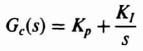
      and is shown in figure P3.2(ii).

      Determine the values of K_p and K_I so that the roots of the characteristic equation are also at −6 and −8.

      

      Figure P3.2(ii)

   5. Which design would you select, the controller configuration of part (a) or the proportional plus integral controller of part (d).
3. 3.3. The controllability and observability of the control system shown in Figure P3.3 is to be determined.

   

   Figure P3.3

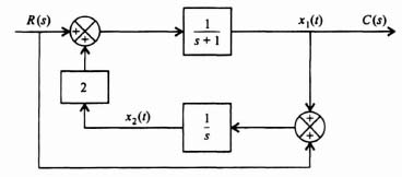
   1. Find the state and output equations of this control system.
   2. Determine the D matrix. Is the system controllable?
   3. Determine the U matrix. Is the system observable?
4. 3.4. Synthesize a system utilizing linear-state-variable feedback that has closed-loop poles existing at −9, 0 and −16, 0 and can satisfy the following specifications:

   

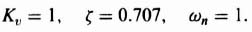
   It is assumed that the process to be controlled has a transfer function given by G(s) = 20/[s(s + 1)(s + 10)], and the transient response is governed by a pair of dominant complex-conjugate poles.

5. 3.5. Repeat Problem 3.4 for the following specifications:

   

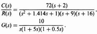
6. 3.6. Repeat Problem 3.4 for the following specifications:

   

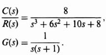
7. 3.7. It is desired to synthesize a system using linear-state-variable feedback which has a closed-loop pole at −4, 0 and can satisfy the following specifications:

   

   It is assumed that the process to be controlled has a transfer function given by

   

   and the transient response is governed by a pair of dominant complex-conjugate poles.

   1. Can the system specifications of velocity constant be met with a simple second-order system?
   2. What must be added to the closed-loop system transfer function?
   3. What must be added to the open-loop system transfer function?
   4. Synthesize the block-diagram configuration of the linear-state-variable feedback configuration for the resulting system.
   5. Determine all unknown network constants and linear-state-variable feedback coefficients.
   6. Draw the root locus, and determine whether the resulting synthesized system is stable. If it shows that the system is unstable, what might be done to stabilize the system?
8. 3.8. It is desired to synthesize a system using linear-state-variable feedback which can satisfy the following specifications:

   

   The process to be controlled has a transfer function given by

   

   and assume that the transient response is governed by a pair of dominant complex-conjugate poles.

   1. Can the system specifications be met with a simple second-order system?
   2. Synthesize the block-diagram configuration of the linear-state-variable feedback for the resulting system.
   3. Determine all unknown constants (if any) and all linear-state-variable feedback coefficients.
   4. Determine whether the resulting synthesized system is stable using the root-locus method for solution.
9. 3.9. Synthesize a system using linear-state-variable feedback that has a closed-loop transfer function given by

   

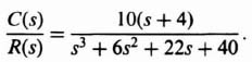
   It is assumed that the process to be controlled has a transfer function given by

   

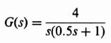
   In your solution, show the following:

   1. Synthesis of the linear-state-variable feedback system.
   2. Identification of any compensation network needed to satisfy the synthesis.
   3. Check of the stability of the resulting system synthesized using the root-locus method.
10. 3.10. A control system is defined by the following:

    

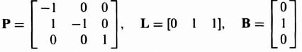
    1. Determine whether the system is controllable.
    2. Determine whether the system is observable.
11. 3.11. The state and output equations of a second-order system are given by the following:

    

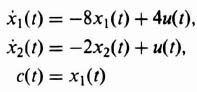
    where x₁(t) and x₂(t) represent the system state, c(t) is its output, and u(t) is its input.

    1. Determine whether the system is controllable.
    2. Determine whether the system is observable.
12. 3.12. A control system is defined by the following:

    

    1. Determine whether the system is controllable.
    2. Determine whether the system is observable.
13. 3.13. Design a second-order controller which is to be critically damped, and whose two second-order roots are located at −7 in the s-plane. The transfer function of the system to be controlled is given by

    

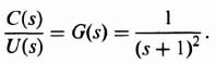
    Find the vector K.

14. 3.14. Repeat Problem 3.13 if the controller is critically damped, but its two second-order roots are now located at −4 instead of −7.
15. 3.15. Design a second-order estimator for a system which is to have a damping ratio of 0.5, and whose estimator has two second-order roots located at −30 in the s-plane. Find the vector M. Assume that ω_n = 1 rad/sec.
16. 3.16. Repeat Problem 3.15 if the two estimator roots are located at −15 instead of −30.
17. 3.17. Design a second-order estimator which satisfies the ITAE criterion for a zero steady-state step error system. Assume that ω_n = 25 rad/sec,
18. 3.18. We wish to design a regulator system (where the reference input equals zero) containing a combined controller and estimator as illustrated in Figure 3.19. The process' transfer function is given by the following expression:

    

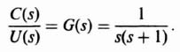
    1. Determine the state and output equations of this process.
    2. We wish to design the controller whose design specifications are for ω_n = 2 rad/sec and for ζ = 1. Determine the controller gain matrix, K.
    3. We wish to design the estimator to have a much faster response than the controller. Therefore, we will design the estimator to have ω_n = 20 rad/sec and ζ = 1. Determine the estimator gain matrix M.
    4. Determine the resulting compensator's transfer function, U(s)/C(s).
    5. We wish to extend the design of this sytem to the case of a system containing a reference input, r(t), as shown in Figure 3.22. Determine the vector N so that the estimator error is independent of r(t). Assume that A = 10.
19. 3.19. Repeat the problem solved in Section 3.6 using Ackermann's Formula for a process transfer function given by

    

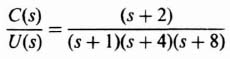
    and the control system's signal-flow graph is shown in Figure P3.19.

    

    Figure P3.19

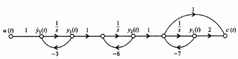
    1. Determine the state equations for the process.
    2. Determine the controllablity matrix for this original system. Is the system controllable?
    3. Transform the original system to the phase-variable form, and determine the state and output equations.
    4. Determine the controllability matrix for the phase variable form.
    5. Determine the transformation matrix A.
    6. Design a controller assuming that the dominant pair of complex-conjugate roots has a damping ratio of 0.707, and it results in a settling time of 4 sec. Select the third pole at the location of the zero of the process to be controlled. What is the resulting characteristic equation of the desired closed-loop control system?
    7. Determine the state and output equations for the phase-variable form with linear-state-variable feedback.
    8. What is the resulting characteristic equation for the set of equations found in part (g)?
    9. Determine the linear-state-variable feedback constants for the control system in phase-variable form.
    10. Transform the linear-state-variable feedback constants back to the original system using the transformation matrix A.
    11. Draw the resulting closed-loop control system with linear-state-variable feedback.
20. 3.20. Determine the closed-loop transfer function of the resulting closed-loop control system developed using Ackermann's Formula and shown in Figure 3.17, and compare it with the desired closed-loop transfer function given by Eq. (3.107). Do they agree?
21. 3.21. The design of the positioning system of a tracking radar is a very interesting control-system problem. Figure P3.21(a) illustrates a tracking radar which has wind torque disturbances acting on it, and the equivalent block diagram for one axis of the tracking radar's positioning loop is illustrated in Figure P3.21(b). The block diagram illustrated represents a two-degrees-of-freedom robust control system which has the dual capability of minimizing the effects of the wind torque disturbance D(s) while also being robust (insensitive) to variations in the gain K. The transfer function for the forward-loop transfer function for the tracking radar G₀(s) is given by

    

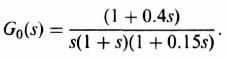
    1. Determine the transient response of this control system to a unit step input at R(s) assuming that G_c1(s) = G_c2(s) = 1 and K has a nominal value of 40, but can also vary as low as 10 and as high as 160.
    2. Draw the root locus for the conditions in part (a). Determine the location of the closed roots for K = 10, 40, and 160, and determine the damping ratio for the dominant complex-conjugate roots for these three cases.
    3. Design G_c2(s) so that it contains the zeros which cancel the complex-conjugate roots for the case of nominal gain 40.

       

       Figure P3.21 A tracking radar conceptually illustrating disturbance torques due to wind forces (a), and the equivalent block diagram of the tracking radar's positioning loop (b).

    4. Draw the root locus for the conditions of part (c). Determine the location of the closed-loop roots for K = 10, 40, and 160, and determine the damping ratio for the dominant complex-conjugate roots for these three cases.
    5. Design the robust controller G_c1(s), and plot the resulting transient response of this control system containing G_c1(s) and G_c2(s), which was designed in part (c).
    6. How do the transient responses of part (e) compare to the transient responses of part (a)? Discuss the robustness of your resulting design to variations in the gain K.
22. 3.22. The optimum sensitivity for the control system illustrated in Figure P3.22 is to be determined in the H^∞ sense. The proces G(s) has a transfer function given by

    

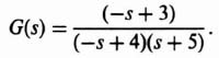
    The weighting function, W(s), is given by

    

    

    Figure P3.22

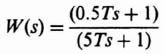
    1. Determine B_p(s).
    2. Determine B'(s).
    3. Determine k.
    4. Determine S(s).
    5. Determine the magnitude of the optimum value of the sensitivity function. |S(jω)|, as a function of T.
    6. From your results for |S(jω)| in part (e), plot the magnitude of the optimum sensitivity function as a function of ω for T = 0.2. 2 and 20.

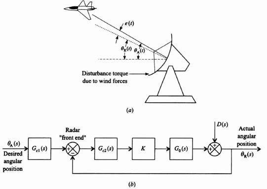
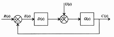
REFERENCES

1. J. L. Melsa and D. G. Schultz, Linear Control Systems. McGraw-Hill, New York, 1969.

2. R. E. Kalman, “On the general theory of control systems.” In Proceedings of the First International Congress of Automatic Control, Moscow, 1960.

3. R. E. Kalman, Y. C. Ho, and K. S. Navendra, “Controllability of linear dynamical systems.” Contrib. Differ. Equat., 189–213 (1961).

4. E. G. Gilbert, “Controllability and observability in multivariable control systems.” J. Control. Ser. (A) 1, Soc. Ind. Appl. Math., 128–151 (1963).

5. J. E. Ackermann, “Der Entwurf Iinearer regelungs Systems in Zustandstraum.” Regelungstech, Prozess-Datenverarb, 7, 297–300 (1972).

6. K. Ogatta, Modern Control Engineering, 3rd ed., Prentice-Hall, Englewood Cliffs, NJ, 1997.

7. N. S. Nise, Conrrol Systems Engineering, 2nd ed., Addison-Wesley, Reading, MA, 1995.

8. G. F. Franklin, J. D. Powell, and A. Emami-Naeini, Feedback Control of Dynamic Systems, 2nd ed. Addison-Wesley, Reading, MA, 1991.

9. A. Emami-Naeini and G. F. Franklin, “Zero assignment in the multivariable robust servomechanism:” Proc IEEE Conf. Dec. Control., 1982. pp. 891–893.

10. Modern CACSD Using the Robust Control Toolbox by R. Y. Chiang and M. G. Safonou, Proc. Conf. on Aerospace and Computational Control, Oxnard, CA, August 28–30. 1989.

11. P. Dorato, Robust Control, IEEE Press, New York, 1987.

12. P. Dorato, “Case Studies in Robust Control Design.” IEEE Proceedings of the Decision and Control Conference, December 1990, pp. 2030–3031.

13. B. C. Kuo, Automatic Control Systems. 7th ed., Prentice-Hall, Englewood Cliffs, NJ, 1995.

14. P. A. Ioannou and J. Sun, Robust Adaptive Control. Prentice-Hall Professional Technical Reference, Des Moines, IA, 1995.

15. J. Ackermann, “Robust Control Prevents Car Skidding.” IEEE Control Systems, 17, pp. 23–31 (1997).

16. G. Zames, “Feedback and Optimal Sensitivity; Model Reference Transformations, Multiplicative Seminonns, and Approximate Inverses,” IEEE Transactions on Automatic Control, AC-26, 301–320 (1981).

17. P. R. Belanger, Control Engineering. Saunders College Publishing, Harcourt Brace and Company, Fort Worth, 1995.

18. Z. Gajic and M. Lelic, Modern Control System Engineering. Prentice-Hall, 1996.

19. B. A. Francis, J. W. Helton, and G. Zames, “H^∞-Optimal Feedback Controllers for Linear Multivariable Systems. IEEE Trans. Automatic Control, AC-29, 888–900 (1984).

20. J. C. Doyle, K. Glover, P. O. Khargonekhav, and B. A. Francis, “State Space Solutions to Standard H² and H^∞ Control Problems.” IEEE Trans. Automatic Control, 34, 831–847 (1989).

21. A. F. A. Serrarens, M. J. G. van de Molengraft, J. J. Kok, and L. van der Steen, “H-Infinity Control for Suppressing Stick-Slip in Oil Well Drillstrings.” IEEE Control Systems, 18–2, 19–30 (1998).

22. A. J. Laub, “Numerical Linear Algebra Aspects of Control Design Computations.” IEEE Trans. Automatic Control, AC-30, 97–108 (1985).

23. K. J. Åström and B. Wittenmark, Computer-Controlled Systems, Theory and Design. Prentice-Hall, Englewood Cliffs, NJ, 1990.

24. A. J. Laub, “Efficient multivariable frequency response calculations.” IEEE Trans. Automatic Control, AC-26, 407–408 (1981).

25. C. B. Moler and G. W. Stewart, “An algorithm for generalized matrix eigenvalue problems.” SIAM J. Numer. Anal., 10, 241–256 (1973).