
5
NONLINEAR CONTROL-SYSTEM DESIGN
5.1. INTRODUCTION
The feedback control-system design methods presented in previous chapters were restricted to linear constant systems, that is, systems that can be represented by linear differential equations with constant coefficients. In practice, linear systems possess the property of linearity only over a certain range of operation; all physical systems are nonlinear to some degree. Therefore it is important that one acquire a facility for analyzing control systems with varying degrees of nonlinearity.
Any attempt to restrict attention strictly to linear systems can only result in severe complications in system design. To operate linearly over a wide range of variation of signal amplitude and frequency would require components of an extremely high quality; such a system would probably be impractical from the viewpoints of cost, space, and weight. In addition, the restriction of linearity severely limits the system characteristics that can be realized.
In practice, linear operation is required only for small deviations about a quiescent operating point. The saturation of amplifying devices having large deviations about the quiescent operating point is usually acceptable. The presence of nonlinearities in the form of dead zones for small deviations about the quiescent operating point is also usually acceptable. In both cases one attempts to limit the effects of nonlinearities to acceptable tolerances, as it is impractical to eliminate the problem entirely.
It is worth noting that nonlinearities may be intentionally introduced into a system in order to compensate for the effects of other undesirable nonlinearities, or to obtain better performance than could be achieved using linear elements only. A simple example of an intentional nonlinearity is the use of nonlinear damping (see Section 4.5‡) to optimize response as a function of the error [1]. The on-off contactor (relay) servo, where full torque is applied as soon as the error exceeds a specified value, is another case of an intentionally nonlinear system.
The purpose of this chapter is to examine the broad aspects of nonlinear systems. We first study the characteristics of nonlinearities and then present several methods for analysis and design of nonlinear control systems. We follow in Chapter 6 with several illustrations of synthesis of nonlinear systems having intentional nonlinearities utilizing optimal control theory. A case study of a positioning system containing nonlinearities is presented in Chapter 7.
We should emphasize here that methods of analyzing nonlinear systems have not progressed as rapidly as have techniques for anlayzing linear systems. Comparatively speaking, at the present time we are still in the development stage. However, the various methods presented in this chapter will enable one to analyze and synthesize nonlinear control systems quantitatively.
5.2. NONLINEAR DIFFERENTIAL EQUATIONS
A linear differential equation of the nth order, with constant coefficients, is written

where x(t) represents the input to the system, t represents time and is the independent variable, y(t) represents the dependent variable, or the output of the system, and An, An–1,…, A0 are constants.
This equation is of the form derived for several representative mechanical and electrical systems in Chapter 3‡. For example, Eq. (3.19)‡, which is repeated below, gave the differential equation of motion for a mechanical system which consists of a force f(t) applied to a mass, damper, and spring:

The mass of the system is represented by the constant M, the damping factor by the constant B, and the spring constant by K.
Detailed solutions for the class of differential equations having the form shown in Eq. (5.1) are available. They have been studied extensively, and several powerful techniques, such as the Laplace transformation, exist for their solution. All the analytical methods discussed in Chapter 1 and Chapter 2 are based on systems that can be represented by simple differential equations having this general form.
If any of the coefficients An, An–1,…, A0 are functions of the independent variable time, then the linear differential equation is said to have variable coefficients. In this case, the differential equation takes the following form:

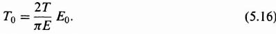
where An, An–1,…, A0 are all functions of time. Except in special cases (such as when the coefficients are polynomials), the solution of linear time-variable equations is quite complex.
If the coefficients of the differential equation are functions of the dependent variable y(t), then a nonlinear differential equation results. Its general form is
where x(t) represents the input to the system, t represents time and is the independent variable, y(t) represents the dependent variable and the output of the system, An, An–1,…, A0 are constants, ![]() is a constant indicating the degree of nonlinearity present, and f(y(t), dy(t)/dt,…, dn–1 y(t)/dtn–1) is a nonlinear function.
is a constant indicating the degree of nonlinearity present, and f(y(t), dy(t)/dt,…, dn–1 y(t)/dtn–1) is a nonlinear function.
Notice that if ![]() = 0, Eq. (5.3) reduces to Eq. (5.1), which represents a linear differential equation having constant coefficients. This leads us to the qualitative rule that a small amount of nonlinearity in a system means that
= 0, Eq. (5.3) reduces to Eq. (5.1), which represents a linear differential equation having constant coefficients. This leads us to the qualitative rule that a small amount of nonlinearity in a system means that ![]() is small in comparison with the coefficients An, An–1,…, A0. In addition, a large amount of nonlinearity means that
is small in comparison with the coefficients An, An–1,…, A0. In addition, a large amount of nonlinearity means that ![]() is large compared with An, An–1,…, A0.
is large compared with An, An–1,…, A0.
5.3. PROPERTIES OF LINEAR SYSTEMS THAT ARE NOT VALID FOR NONLINEAR SYSTEMS
Several inherent properties of linear systems, which greatly simplify the solution for this class of systems, are not valid for nonlinear systems. The fact that nonlinear systems do not have these properties further complicates their analysis.
Superposition is a fundamental property of linear systems. As a matter of fact, this property is the basis of the definition of a linear system. The principle of superposition states that if c1(t) is the response of a system to r1(t) and c2(t) is its response to r2(t), then the system's response to a1r1(t) + a2r2(t) is a1c1(t) + a2c2(t). Unfortunately, the superposition principle does not apply to nonlinear systems. Therefore, several mathematical procedures used in the design of linear systems cannot be used for nonlinear systems.
Stability of linear systems has been shown (in previous chapters) to depend only on the system's parameters. The stability of nonlinear systems, however, depends on the intial conditions and the nature of the input signal as well as the system parameters. One cannot expect a nonlinear system that exhibits a stable response to one type of input to have a stable response to other types of input. We shall shortly illustrate nonlinear systems that are stable for very small or very large signals, but not for both.
We normally expect the output of a linear system, excited by a sinusoidal signal, to have the same frequency as the input, although its amplitude and phase may differ. However, the output of nonlinear systems usually contains additional frequency components and may, in fact, not contain the input frequency.
For linear systems, interchanging two elements in cascade does not affect behavior. This is not true if one of the elements is nonlinear.
The question of stability is clearly defined for linear constant systems: A system is either stable or unstable. An unstable linear constant system has an output that grows without bound, either exponentially or in an oscillatory mode with the envelope of the oscillations increasing exponentially. In the nonlinear systems, system instability may means a constant-amplitude output having an arbitrary waveform. It is important to emphasize that an oscillator is stable according to Liapunov [2, 3]. The exponentially decaying system, which we have referred to in this book as being stable, is described by Liapunov as being asymptotically stable.”*
5.4. UNIQUE CHARACTERISTICS OF NONLINEAR SYSTEMS
This section describes in detail some of the unusual characteristics that are peculiar to nonlinear systems. These phenomena, which do not occur in linear systems, may be desirable or undesirable depending on the application. We discuss specifically the following behavior: limit cycle, soft and hard self-excitation, hysteresis, jump resonance, and subharmonic generation.
Limit cycles are oscillations of fixed amplitude and period that occur in nonlinear systems. Depending on whether the oscillation converges or diverges from the conditions represented, limit cycles can be either stable or unstable. It is possible that conditionally stable systems may contain both a stable and an unstable limit cycle. The occurrence of limit cycles in nonlinear systems makes it necessary to define instability† in terms of acceptable magnitudes of oscillation, because a very small nonlinear oscillation may not be detrimental to the performance of a system.
Self-excited oscillations occurring in systems that are unstable in the presence of very small signals are called soft self-excitation. Self-excited oscillations occurring in systems that are unstable in the presence of very large signals are called hard-self-excitation. Because soft and hard types of oscillation can occur, the control engineer must specify the dynamic range of operation completely when designing a nonlinear system. A feedback control system containing an element having saturation characteristics, such as illustrated in Figure 5.1a, could exhibit soft self-excitation. A feedback control system containing an element having dead-zone characteristics, such as illustrated in Figure 5.1b, could exhibit hard self-excitation.
Hysteresis is a nonlinear phenomenon that is most usually associated with magnetization curves or backlash of gear trains. A conventional magnetization curve whose path depends on whether the magnetizing force H is increasing or decreasing is shown in Figure 5.1c.
Jump resonance [4], another form of hysteresis, is of considerable interest. It exhibits itself in the closed-loop frequency response of certain nonlinear systems, as illustrated in Figure 5.1d. As the frequency ω is increased and the input amplitude R is held constant, the response follows the curve AFB. At point B, a small change in frequency results in a discontinuous jump to point C. The response then follows the curve to point D upon further increase in frequency. As the frequency is decreased from point D, the response follows the curve to points C and E. At point E, a small change in frequency results in a discontinuous jump to point F. The response follows the curve to point A for further decreases in frequency. Observe from this description that the response never actually follows the segment BE. This portion of the curve represents a condition of unstable equilibrium. The system must be of second order or higher for the phenomenon of jump resonance to occur.
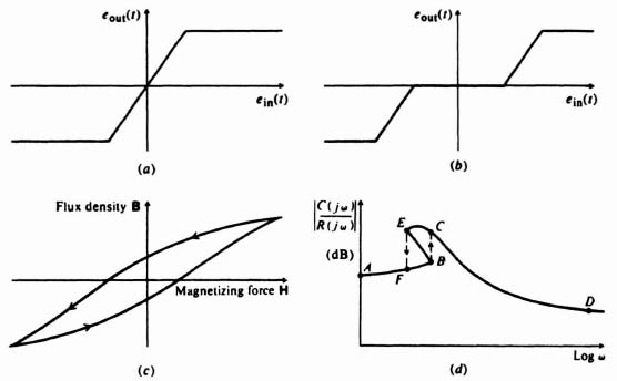
Figure 5.1 (a) Saturation characteristics. (b) Dead-zone characteristics. (c) Conventional hysteresis loop. (d) Closed-loop response of a system with jump resonance.
Subharmonic generation [5] refers to nonlinear systems whose output contains subharmonics of the input's sinusoidal excitation frequency. The transition from normal harmonic operation to subharmonic operation is usually quite sudden. Once the subharmonic operation is established, however, it is usually quite stable. In general, if sinuosoidal signals f1 and f2 are added and their sum is applied to a nonlinear device, the output contains frequency components af1 ± bf2, where a and b assume all possible integers includingzero.
5.5. METHODS AVAILABLE FOR ANALYZING NONUNEAR SYSTEMS
Several tools are available for the analysis of nonlinear systems. All these techniques depend on the severity of the nonlinearity and/or the order of the system under consideration. We consider all of the useful and popular techiques in this chapter and illustrate their practical application. The chapter concludes with the presentation of guidelines for selecting the “best” nonlinear control-system method for the analysis and design of a particular problem in Section 5.23.
The analysis of nonlinear systems is concerned with the existence and effects of limit cycles, soft and hard self-excitation, hysteresis, jump resonance, and subharmonic generation. In addition, the response to specific input functions must be determined, The major difficulty of analyzing nonlinear systems is that no single technique is generally applicable to all problems.
Quasilinear systems, where the deviation from linearity is not too large, permit the use of certain linearizing approximations [6]. The describing-function approach, which is applicable to nonlinear systems of any order and is concerned with discovering limit cycles, simplifies the problem by assuming that the input to the nonlinear system is sinusoidal and the only significant frequency component of the output is that component having the same frequency as the input [7–10].
Nonlinear systems can often be approximated by several linear regions: The piecewise-linear approach permits the segmented linearization of any nonlinearity for any order of system. The phase-plane method is a very useful technique for analyzing the response of a second-order nonlinear system [10–13]. Liapunov's stability methods are very powerful techniques for determining the steady-state stability of nonlinear systems based on generalizations of energy notions [2]. Popov's method is very useful for determining the stability of time-invariant, nonlinear systems. The generalized circle criterion is applicable to time-variable, nonlinear systems whose linear portion is not necessarily open-loop stable [16,17].
Systems of very high order having several nonlinearities have hardly been dealt with in general analytical terms, This problem usually requires the use of numerical methods utilizing digital computers for a solution. It is worth emphasizing at this point that any nonlinear differential equation can be solved by these techiques provided many small increments are used [21–24]. However, the resulting solution is valid only for the specific problem being considered. It is very difficult to extend the result and obtain a general solution which can be used for other problems.
As a final check on the stability of nonlinear control systems, I always recommend that the system be simulated [25,26]. It will aid in overcoming such factors as possible uncertainty regarding the validity of assumptions, and to analytic difficulties caused by system complexity. That is further emphasized in Section 5.23.
5.6. UNEARIZING APPROXIMATIONS
In quasilinear systems, where the deviation from linearity is not too great, linear approximations may permit the extension of ordinary linear concepts. This approach acknowledges that certain system characteristics change from operating point to operating point, but it assumes linearity in the neighborhood of a specific operating point. The technique of linearizing approximations is universally used by the engineer and may be more familiar to the reader under the names small-signal theory and/or theory of small perturbations.
Linearizing approximations were utilized when we discussed the two-phase ac servomotor in Section 3.4‡. For this device, Figure 3.16‡ illustrated the quasilinear characteristics relating developed torque and speed. However, by approximating the torque speed curves with straight lines, the linear differential equation (3.98)‡ was formulated. We then obtained the transfer function of the two-phase ac servomotor, assuming that it was a linear device. It is left as an exercise to the reader in Problem 5.1 to determine the effect of various linearizing approximations.
The effects of a small amount of nonlinearity can be studied analytically by considering small perturbations or changes in the variables about some average value of the variables. This can be represented analytically by [see Eq. (5.3)]
An expansion of the solution to this differential equation, for small nonlinearities, can be written as a power series in ![]() as
as
From this equation, y(t) may be interpreted as being composed of a linear component y(0)(t) and several deviation factors: ![]() . Assuming that
. Assuming that ![]() is very small, the nonlinear components will not seriously affect the system's behavior if a linear approximation is assumed. Therefore, within the realm of reasonable engineering approximations, the control engineer may be able to extend linear theory for certain feedback control systems which exhibit a small amount of nonlinearity. It is very interesting that this is just the reason linear theory has had such good results, even though practical systems are never purely linear.
is very small, the nonlinear components will not seriously affect the system's behavior if a linear approximation is assumed. Therefore, within the realm of reasonable engineering approximations, the control engineer may be able to extend linear theory for certain feedback control systems which exhibit a small amount of nonlinearity. It is very interesting that this is just the reason linear theory has had such good results, even though practical systems are never purely linear.
Linearization techniques can also be applied to those problems where it is desired to linearize nonlinear equations by limiting attention to small perturbations about a reference state [6]. This technique is often used in the design of space navigation and control systems where it is desired to maintain a space vehicle along a specified reference trajectory. It will now be shown how the corrective control forces required to keep the vehicle on the desired flight trajectory can be synthesized from a set of linear differential equations, although the basic differential equations describing the reference flight trajectory are nonlinear.
To illustrate this, let us assume that the equation of the system is given by
where the function f is nonlinear. Figure 5.2 illustrates the reference trajectory of the space vehicle (solid line) which satisfies the equation
where the superscript zero refers to parameters occurring along the reference trajectory. These reference parameters are related to the parameters of the actual trajectory (dashed line) as follows:
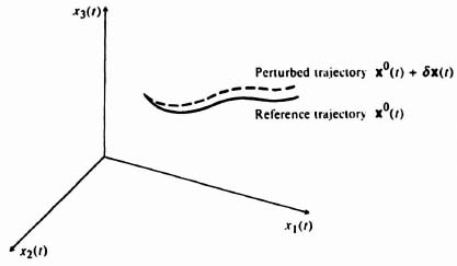
Figure 5.2 Reference and perturbed trajectories of a space vehicle [6].
Figure 5.2 illustrates the reference and actual trajectories, where the actual state x(t) is perturbed from the reference state x0(t) by δx(t). Physically, this means that the actual trajectory of the space vehicle is perturbed, or slightly different, from that of the desired reference trajectory. The vector δu(t) represents the deviation of the control input from the desired reference input u0(t) which would result in the desired system response x0(t).
What kind of relationship can we derive between x0(t), δx(t), u0(t), and δu(t)? The basic nonlinear equation of the system,
![]()
can be expressed as

Because we are assuming that the actual perturbations of the system are small, we can expand the jth component of this equation in a Taylor series about the reference trajectory as follows:
Using Eq. (5.7), we can rewrite Eq. (5.10) as follows:

where j = 1, 2, 3,…, m.
Equation (5.11) can be simplified by utilizing the Jacobian matrices* that are defined as follows:

It is important to emphasize that all of the partial derivatives in the Jacobian matrices are evaluated along the reference trajectory of the space vehicle. Based on the Jacobian matrices, Eq. (5.11) can be rewritten in the following simplified form:
This resulting equation is very important. It states that the differential equation describing the perturbations about the reference trajectory are approximately linear, although the basic system differential equations describing the reference flight trajectory are nonlinear. Therefore, we have succeeded in linearizing the problem.
We can also linearize a system if we can adapt it to behave like a linear system. In order to demonstrate this, let us consider a two-position relay that controls the rotation of a motor in either direction. It is assumed that the control voltage applied by the relay to the motor, ec(t), is given by
and the resulting motor torque developed, T(t), would be a square wave due to the switching action. Both ec(t) and T(t) are illustrated in Figure 5.3. Observe from this figure that the average, or mean, value of both functions is zero.
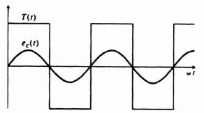
Figure 5.3 Relay-conlrolled molar characlerislics—Case 1.
Let us next assume that the control voltage has a finite mean value E0, where
For this case, the torque is a periodic function whose mean value is some nonzero value T0, because time intervals where ec(t) is positive or negative are not equal, as indicated in Figure 5.4. Note that E0 is also a function of time, but it is assumed that it is very slowly varying compared with ω. Assuming, in addition, that E0 ![]() E, it can easily be shown that the mean value of T0 is given by the linear relationship
E, it can easily be shown that the mean value of T0 is given by the linear relationship
Therefore, the mean value of the torque T0 is proportional to the mean value of the controlling voltage.
This is a very important result. It shows that by means of a nonlinear element like a relay, a linear relationship can be obtained between the mean value of the controlling voltage and the mean value of the motor torque developed. The basic linearization technique utilized has taken the mean value of the applied voltage to the relay as the input, and superimposed on it a sinuosidal function of time whose amplitude and frequency are very high relative to that of the input.
In the following section, we extend our linearization concepts and attempt to apply them to nonlinear systems. Although the notion of a transfer function is inapplicable for nonlinear systems, an equivalent approximate transfer characteristic for a nonlinear device can be derived which can be manipulated as a transfer function under certain circumstances. We define this approximate transfer characteristic as the describing function. It is a very useful notion and is frequently employed in practice.
5.7. DESCRIBING-FUNCTION CONCEPT
The use of describing functions is an attempt to extend the very powerful transfer-function approach of linear systems to nonlinear systems [7, 8, 10]. A describing function is defined as the ratio of the fundamental component of the output of a nonlinear device to the amplitude of a sinusoidal input signal. In general, the describing function depends on the input signal's amplitude and frequency and is complex because phase shift may occur between the input and the fundamental component of the output. We study the describing function method of analysis and compare it with the transfer-function concept for linear systems.
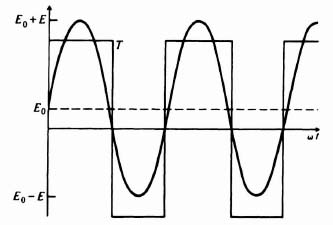
Figure 5.4 Relay-controlled motor characteristics—Case 2.
If the input to a nonlinear element is a sinusoidal signal, the describing-function analysis assumes that the output is a periodic signal having the same fundamental period as that of the input signal. Therefore, the analysis is concerned only with the fundamental component of the output waveform. All harmonics, subharmonics, and any de component are neglected. This assumption is reasonable, because the harmonic terms are often small when compared with the fundamental term. In addition, a feedback control system usually provides additional attenuation of the harmonic terms because of its inherent filtering action of high frequencies in the region of the harmonic terms. Many nonlinear elements do not generate a dc term because they are symmetrical, nor do they generate any subharmonic terms [5]. Therefore, in many (but not all) situations the fundamental term is the only significant component of the output of the nonlinear element. In addition, it is assumed that there is only one nonlinear element in the feedback control system and that it is not varying. If a system contains more than one nonlinearity, we must lump all the nonlinearities together and obtain an overall describing function.
An examination of these limitations indicates that the describing function is based on a restricted mathematical foundation. The technique does give, however, reasonable results and does have an advantage that it can be used for systems of any order and is fairly simply to apply. It is recommended that the results always be verified with another technique or a computer simulation [25,26].
Given its limitations, the describing-function technique is still a very useful tool for analyzing and designing nonlinear systems. The describing function should be thought of as a generalized transfer function for nonlinear systems.
In order to derive a mathematical expression for the describing function, let us consider the general nonlinear system illustrated in Figure 5.5. In accordance with the definition of the describing function, let us assume that the input to the nonlinear element N(M, ω) is given by
In general, the steady-state output of the nonlinear device can be represented by the series
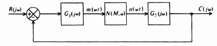
Figure 5.5 General nonlinear system.
By definition, the describing function is

Notice that the describing function depends on the amplitude and frequency of the input signal. The nonlinear element is thus considered to have a gain and phase shift varying with the amplitude and frequency of the input signal.
5.8. DERIVATION OF DESCRIBING FUNCTIONS FOR COMMON NONLINEARITIES
The describing functions for several common nonlinearities are derived in this section [8–10, 27]. The procedure most commonly used is to determine the Fourier series of the output waveshape from the nonlinear device and consider only the fundamental component. Let us consider the nonlinear element N(M, ω) in an overall feedback control system, as shown in Figure 5.5. Assuming that the input m(ωt) is given by a sinusoidal signal where
we can represent the output waveshape by a Fourier series given by the expression

where


In general, if n(ωt) = −n(−ωt), then the function is odd and AK = 0. In addition, if n(ωt) = n(−ωt), then the function is even and BK = 0.
Because we are only concerned with the fundamental component of the output, it is necessary to determine only A1 and B1. For m(ωt) = M sin ωt, the describing function can then be obtained from the expression

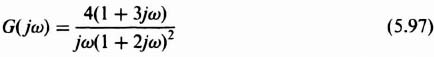
The control engineer is usually concerned with the nonlinearities due to dead zones, saturation, backlash, on-off relay-control systems, Coulomb friction, and stiction. We specifically derive and catalog their describing functions so that a handy reference for some common describing functions will be available. In addition, the procedure illustrated should enable one to develop the facility for calculating the describing function of any nonlinearity encountered.
A. Describing function of a Dead Zone
Figure 5.6 illustrates the dead-zone characteristics. The relationships between input and output of this nonlinearity can be expressed by the equations
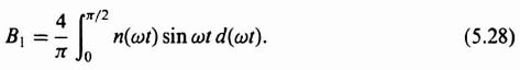
Figure 5.7 illustrates typical input and output waveshapes. Notice that the output is an odd function, and therefore AK = 0. The symmetry over the four quarters of the period allows us to evaluate the expression for the Fourier coefficient, B1, by taking four times the integral over one quarter of a cycle, as follows:
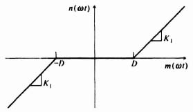
Figure 5.6 Nonlinear characteristics of a dead zone.

Figure 5.7 Input and output waveshape from a nonlinear device having the dead-zone characteristics shown in Figure 5.6.
Substituting Eqs. (5.25) and (5.26) into Eq. (5.28), we obtain

where
![]()
Evaluation of Eq. (5.29) results in the expression

From Eq. (5.30), because the describing function is the ratio of the amplitude of the fundamental component of the output B1 to M, it can be expressed as

Notice that the describing function for a dead zone is only a function of the amplitude of the input and not of frequency. Figure 5.8, obtained from Eq. (5.31), is a sketch of the normalized value of the describing function N(M)/K1 as a function of the ratio D/M. For very small values of D/M the normalized describing function approaches unity. For values of D/M ![]() 1 it equals zero, which implies that the input must be greater than the dead-zone magnitude in order to obtain an output. Notice that the describing function for a dead zone does not have any phase shift.
1 it equals zero, which implies that the input must be greater than the dead-zone magnitude in order to obtain an output. Notice that the describing function for a dead zone does not have any phase shift.
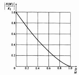
Figure 5.8 Normalized describing function for a dead zone.
B. Describing function of Saturation
Figure 5.9 illustrates the nonlinear saturation characteristic. The relationship between input and output of this nonlinearity can be expressed by the following equations

Figure 5.10 illustrates typical input and output waveshapes.

Figure 5.9 Nonlinear characteristics of saturation.
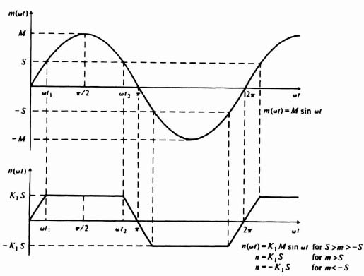
Figure 5.10 Input and output waveshape from a nonlinear device having saturation characteristics shown in Figure 5.9.
Notice that the output waveshape is an odd function for the case of saturation just as it was for the case of a dead zone. Therefore, the expression for the Fourier coefficient B1 of the output waveshape is
As was true for a dead zone, the expression for the Fourier coefficient B1 can be obtained by taking four times the integral over one quarter of a cycle because of the symmetry over the four quarters of the period. This results in the expression

Substituting Eqs. (5.32) and (5.33) into Eq. (5.35), we obtain

where
Evaluation of Eq. (5.36) results in the expression
Because the describing function is defined as the ratio of the amplitude of the fundamental component of the output, B1 to M, the describing function can be expressed as

Notice that the describing function for saturation is only a function of the amplitude of the input and not of frequency. Figure 5.11, obtained from Eq. (5.38) is a sketch of the normalized value of the describing function N(M)/K1 as a function of the ratio S/M. For very small values of S/M, the normalized describing function approaches zero. For values of S/M ![]() 1 it equals unity, which implies that the output is unaffected by the saturation level if S
1 it equals unity, which implies that the output is unaffected by the saturation level if S ![]() M. Notice that the describing function for saturation does not introduce any phase shift.
M. Notice that the describing function for saturation does not introduce any phase shift.
It is important to emphasize that the describing functions for dead zone and saturation could have been obtained from one nonlinear characteristic containing both types of nonlinearities. Then the resulting describing function could be reduced to the describing function of dead zone [Eq. (5.31)] by letting the saturation level approach infinity, or it could be reduced to the describing function of saturation [Eq. (5.38)] by letting the dead-zone width approach zero. It is recommended that the reader derive Eqs. (5.31) and (5.38) using this approach (see Problem 5.2).

Figure 5.11 Normalized describing function for saturation.
C. Describing function of Backlash
Backlash or mechanical hysteresis is due to the difference in motion between an increasing and a decreasing output. Figure 5.12 illustrates a model of backlash, and Figure 5.13 illustrates its characteristics. The source of backlash that usually receives the most attention is the “looseness” inherent in mechanical gearing.

Figure 5.12 Physical model of backlash.

Figure 5.13 Characteristics of backlash.
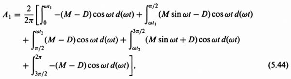
From Figure 5.14, the relationship between inut and output for this nonlinearity can be expressed by the following equations:

Figure 5.14 Backlash characteristics where D < M < 2D.
Notice that the output waveshape is neither an odd nor an even function. This means that the Fourier series of the output waveshape has AK and HK components. Because the describing function is concerned only with the fundamental component of the output, however, we are interested only in A1 and B1. From Eqs. (5.39) through (5.43), we can express A1 as
where

and
and B1 can be expressed as

Integrating Eqs. (5.44) and (5.47), we obtain the following results:


Therefore, the describing function for backlash is given by
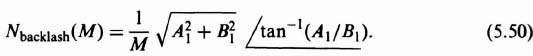
This expression is valid only when the positive slope of the backlash characteristic as shown in Figure 5.14 is unity. If it is any other value, such as K1, then Eq. (5.50) is modified, because the right-hand sides of the defining equations (5.40) and (5.42) would have to be modified.
Notice the describing function for backlash is only a function of the amplitude of the input and not of the frequency. Figures 5.15 and 5.16, which have been obtained from Eqs. (5.48) through (5.50), are sketches of the amplitude and phase characteristics, respectively, of the describing function as a function of the ratio D/M. Notice that a phase lag occurs at low input amplitudes. This phase lag may introduce problems of stability in a feedback system.
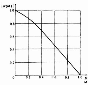
Figure 5.15 Amplitude characteristics for the describing function of backlash.
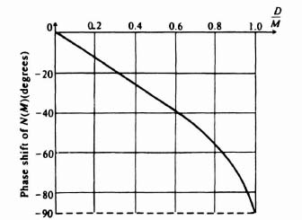
Figure 5.16 Phase characteristics for the describing function of backlash.
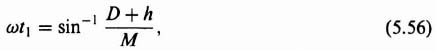
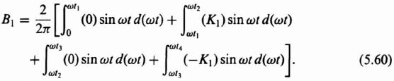
D. Describing function of an On-Off Element Having Hysteresis
A class of systems of great practical importance is that of on-off control systems. In these systems, as soon as the error signal exceeds a certain level, a relay switches on full corrective torque having proper polarity. When the error falls below a certain level, all the corrective torque is removed. These simple and relatively inexpensive devices find many practical uses in thermostatic control of heat, in automobile voltage regulators, in aircraft and space-vehicle control applications where space and weight limitations are very critical, and so on.
The heart of an on-off control system, the relay or contactor, has a variety of characteristics. For the purpose of deriving a describing function, we consider a three-position contactor exhibiting hysteresis characteristics; this includes the two-position contactor as a limiting case. Figure 5.17 illustrates the input-output characteristic and the waveshapes for such a device. The hysteresis effect occurs because of the different values of control signal required for corrective torque application and its removal. Torque is applied when the control signal reaches ±(D + h), but it is not removed until the control signal equals ±D. The relationship between input and output for this nonlinearity can be expressed by the following equations:
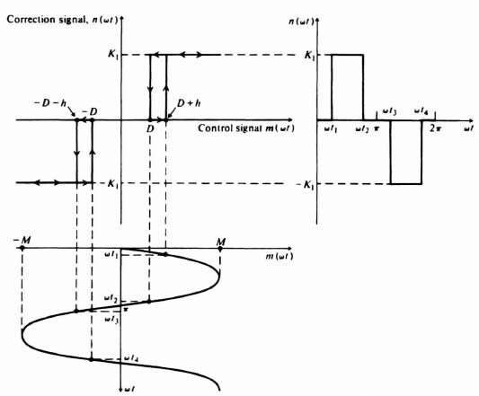
Figure 5.17 On-off characteristics for a three-position contactor having hysteresis.
Notice that the output waveshape is neither an odd nor an even function. The Fourier series of the output waveshape, therefore, contains AK and BK components. From Eqs. (5.51)–(5.54), we can express A1 as

where
and B1 as
Integrating Eqs. (5.55) and (5.60), we obtain the expressions


The describing function is given by the expression
Notice that the describing function for this device is a function only of the amplitude of the input and not of frequency. Figures 5.18 and 5.19, which have been obtained from Eqs. (5.61) and (5.62), are sketches of the normalized amplitude and phase characteristics of the describing function as a function of the ratio M/D, respectively. Notice that the phase lag is zero when hysteresis is not present and grows progressively worse as the hysteresis increases.
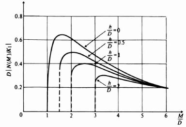
Figure 5.18 Amplitude characteristics for the describing function of an on-off device having hysteresis.
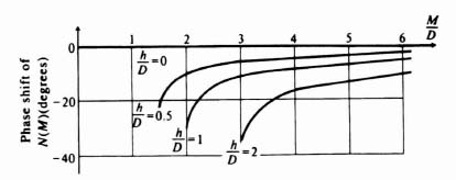
Figure 5.19 Phase characteristics for the describing function of an on-off device having hysteresis.
E. Describing Function of Coulomb Friction and Stiction
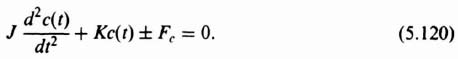
In Chapter 3‡ we considered the effect of damping in linear systems. Damping, a form of friction, is known as viscous friction. Its characteristic is that its magnitude is always proportional to velocity, as illustrated in Figure 5.20a. The damping factor B is the slope of this characteristic. Another type of frictional force commonly found in control systems is known as Coulomb friction. Unlike viscous friction, it is not proportional to velocity but is a constant force that always opposes the velocity. This nonlinear phenomenon is illustrated in Figure 5.20b, where the Coulomb friction force is denoted by ±Fc. Another nonlinear form of frictional force, known as static friction or stiction, is the value of the frictional force at zero velocity. It is usually denoted by ±Fs. Figure 5.20c illustrates the composite frictional-force characteristics generally encountered when controlling some load.
To determine the describing function of Coulomb friction, we can express the relationship between the input and output as

Figure 5.20 (a) Viscous friction characteristics. (b) Coulomb friction characteristics. (c) Composite friction characteristics illustrating viscous, Coulomb, and static friction (stiction).
where
The corresponding steady-state waveforms are given by Figure 5.21. It should be noted that the discontinuities of the output waveform correspond to zero velocity, because the force required to overcome Coulomb friction changes sign at these instants. The relationship between the input and output forces is
where
![]()

Figure 5.21 Coulomb friction characteristics.
The fundamental components of the output A1 and B1 are
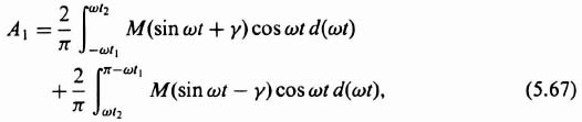
Integrating Eqs. (5.67) and (5.68), we obtain the following expressions:

The resulting expression for Coulomb friction is
Observe that the describing function for Coulomb friction depends only on the amplitude of the input and not on its frequency. The gain-phase relationship of the describing function for Coulomb friction is illustrated in Figure 5.22.
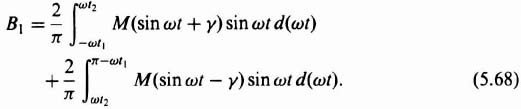
The describing function for the simultaneous occurrence of both Coulomb friction and stiction is considered next. Waveform relationships between the applied force m(ωt), the output force n(ωt), and the forces necessary to overcome Coulomb friction and stiction Fc and Fs are given in Figure 5.23. The expressions for the fundamental components of the Fourier coefficients are

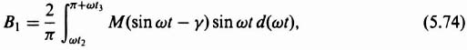
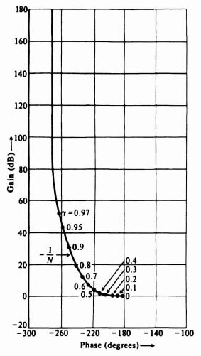
Figure 5.22 Gain-phase characteristics for the describing function of Coulomb friction.

Figure 5.23 Couloumb friction and stiction characteristics.
where

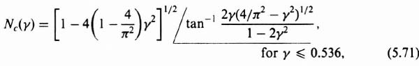
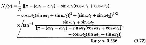
The describing function for the combined case of Coulomb friction and stiction is obtained by integrating Eqs. (5.73) and (5.74). The resultant expression is

Observe from this expression that the describing function for the combined case of Coulomb friction and stiction is a function of the amplitude of the input and the relative magnitudes of friction but not of frequency. Figure 5.24 illustrates the gain-phase relationship of the describing function for the combined case of Coulomb friction and stiction.
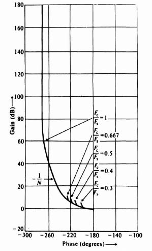
Figure 5.24 Gain-phase characteristics for the describing function of Coulomb friction and stiction.
5.9. USE OF THE DESCRIBING FUNCTION TO PREDICT OSCILLATIONS
The describing function of a nonlinear element can be utilized to determine the existence of a limit cycle in a nonlinear control system in an approximating manner [28]. Let us reconsider the general nonlinear system illustrated in Figure 5.5. If we assume that the describing function of the nonlinearity is N(M, ω) and R(jω) = 0, let us determine the conditions under which an assumed oscillation m(ωt) can be sustained, where
The fundamental component of n(ωt) is given by
Expressing Eqs. (5.76) and (5.77) as the real part of a complex exponential, we obtain the following expressions:
The output of the linear elements is given by
where
Equation (5.78) must equal −m(ωt) if the initial assumption is to hold. Thus, dropping the real-part notation, we obtain the following expression:
![]()
This can be rewritten as
For a sustained oscillation, the bracketed term in Eq. (5.79) must vanish, since M ≠ 0. Therefore,
and any combination of values of input ampitude M and frequency ω which satisfy the equation

are capable of providing a limit cycle. If a combination of amplitude and frequency can be found which satisfies Eq. (5.81), the feedback control system can have a sustained oscillation.
From experience, I have found the gain-phase plot to be the most revealing technique for stability analysis when utilizing the describing-function method. Two separate sets of loci, corresponding to G(jω) and −1/N(M, ω) of Eq. (5.81), are sketched on the gain-phase plot. Intersections of the two loci indicate possible solutions to Eq. (5.81) and yield information as to the magnitude and frequency ω of sustained oscillation. If no intersections result, an oscillation is unlikely. (Remember, the describing function is an approximation.) The distance to a possible intersection can be used as a criterion of closeness to oscillation. This is next illustrated on the gain-phase diagram for several representative systems.
A. Example 5.9-1
Figure 5.25a illustrates an analysis via the gain-phase diagram for a nonlinear system containing a dead zone where K1 = 1. The figure illustrates a stable system where a dead zone is present and

Figure 5.25b illustrates a system where a dead zone is pre sent and

An intersection occurs at a frequency of approximately 4.4 rad/sec and a value of D/M of 0.09. This is to be interpreted as the frequency and amplitude which satisfy Eq. (5.81) and which result in a limit cycle. Notice that the system is unstable from a linear viewpoint, because the −1, 0 point is enclosed.
The interpretation of this situation is quite illuminating. Because the normalized describing function of a dead zone is less than one, its effect is to reduce the overall system gain. When multiplied by the transfer function given by Eq. (5.82), which would produce a stable feedback system by itself, its effect is to make the system even more stable. Therefore, in order to illustrate a limit cycle in this nonlinear system containing a dead zone, it is necessary to illustrate a system that produces an unstable control system from a linear viewpoint as well. The frequency function of Eq. (5.83) satisfies this requirement, as indicated in Figure 5.25b.
It is interesting to observe that this nonlinear control system can only be unstable if we also make it unstable from a linear viewpoint. The next question to answer is how will it behave in an unstable mode, from the linear or nonlinear aspect? A linear system that is unstable has an unbounded response to a bounded input. (Review the BIBO concept presented in Section 6.1.‡) A nonlinear system that is unstable can have a stable or unstable limit cycle. The limit cycle in this problem is a stable one, based on the rule presented in the following problem (see Figure 5.27). Therefore, nonlinear theory states that the system would oscillate at a fixed frequency wand amplitude M defined by the intersection of the two curves in Figure 5.25b. However, linear theory states that the system would have an unbounded output to any bounded input (including noise), and the linear theory viewpoint would be dominant in this problem.

Figure 5.25 (a) Gain-phase diagram stability analysis of nonlinear system containing a dead zone, where

(b) Gain-phase diagram stability analysis of nonlinear system containing a dead zone, where
![]()
B. Example 5.9-2
Figure 5.26 illustrates the gain-phase diagram analysis for a nonlinear system containing backlash, where
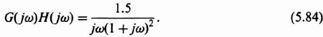

Figure 5.26 Gain-phase diagram analysis of nonlinear system containing backlash.
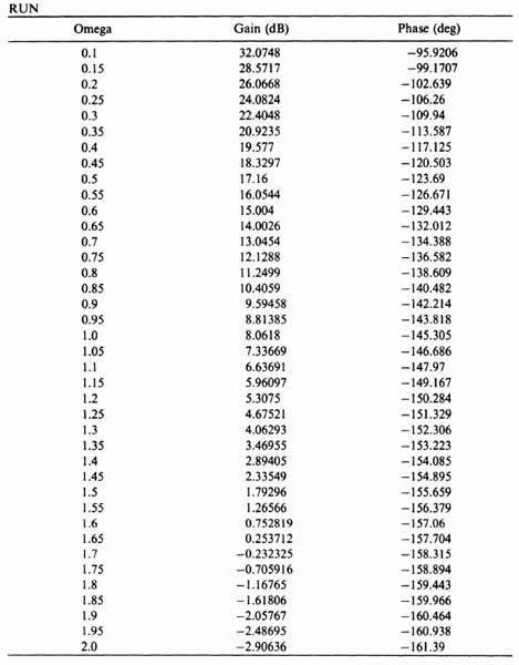
This gain-phase diagram was obtained using MATLAB, [29–31] and is contained in the M-file that is part of my AMCSTD Toolbox disk which can be retrieved free from The MathWorks, Inc. anonymous FTP server at ftp://ftp.mathworks.com/pub/books/advshinners. Notice that the system has two points of intersection corresponding to a pair of limit cycles. They occur at ω = 0.8139, D/M = 0.1742 and ω = 0.2786, D/M = 0.8398. These two limit cycles must now be examined to determine whether they are stable or unstable.
A generalized rule can be established for determining whether a limit cycle is stable or unstable [32]. If the two loci are assigned a sense of direction so that the linear locus G(jω) is pointing in the direction of increasing frequency and the nonlinear locus −1/N is pointing in the direction of increasing amplitude M (decreasing D/M in our example), then a stable limit cycle occurs when the nonlinear locus appears to an observer, stationed on the linear locus and facing in the direction of increasing frequency, to cross from left to right in the direction of increasing amplitude M. If the opposite occurs, then the limit cycle is unstable and the state of the system is divergent. As an example of applying this rule, consider the gain-phase plot of Figure 5.27. Here, we see that there are two unstable limit cycles (divergent states) and three stable limit cycles (convergent states). The unstable limit cycles cannot maintain themselves in the presence of minute disturbances; the stable limit cycles will always maintain themselves in the presence of disturbances.
Applying this generalized rule for determining whether the limit cycles in Figure 5.26 are stable or unstable, we find that ω = 0.8139, D/M = 0.1742 corresponds to a stable limit cycle and the other intersection corresponds to an unstable limit cycle. The stable limit cycle corresponds to a convergent point because disturbances at either side tend to converge to these conditions. This is contrasted with the unstable limit cycle at ω = 0.2786, D/M = 0.8398, which is a divergent point, because disturbances that are not large enough to reach this intersection will decay, and disturbances that are larger will result in oscillations that tend to increase in amplitude until the stable limit cycle is reached.

Figure 5.27 Illustration of stable and unstable limit cycles.
The describing function analysis presented in this book uses the following special functions, which are part of my AMCSTD Toolbox: relays;back_lsh.m;dead_zn.m. They determine the following:
- back_lsh.m determines the value of N(M) in Eq. (5.50) for the describing function of backlash, and is then used for the gain-phase plot. Values of D/M and ω at the various limit-cycle intersections, if any, are then provided as an output after the values for the linear transfer function, G(jω), and an initial estimate of where D/M is at the intersection are provided as inputs to BACK_LSH.M.
- dead_zn.m determines the value of N(M) in Eq. (5.31) for the describing function of dead zone, and is then used for the gain-phase plot. Values of D/M and ω at the various limit-cycle intersections, if any, are then provided as an output after the values for the linear transfer function, G(jω), and an initial estimate of where D/M is at the intersection are provided as inputs to dead_zm.m.
- relays determine the value of N(M) in Eq. (5.63) for the describing function of an on-off element having hysteresis, which can be used for the gain-phase plot. Values at the various limit cycle intersections, if any, can be determined after the values for the linear transfer function, G(jω), are added to the gain-phase plot.
The calculations performed in back_lsh.m and dead_zn.m are based on the describing function definitions, and are analytical and very accurate as opposed to those results obtained using graphical techniques. The determination of N(M) by relays for a nonlinear on-off element having hysteresis is based on this nonlinear device's describing-function definition, but the solution for limit cycles using relays is based on graphical techniques. These three functions could be used as illustrations by the student to implment functions for the other nonlinear characteristics presented (e.g., saturation). My AMCSTD Toolbox can be retrieved free from The MathWorks, Inc. anonymous FTP server at ftp://ftp.mathworks.com/pub/books/advshinners.
5.10. COMPENSATION AND DESIGN OF NONLINEAR CONTROL SYSTEMS USING DESCRIBING FUNCTIONS
The purpose of this section is to illustrate the procedure for compensating for undesirable nonlinearities in a system. As an example, we consider the nonlinearity to be backlash. The gain-phase plot will be used for analysis, although we could use the Nyquist diagram just as well.
Oscillating input signals, having frequencies very much greater in magnitude than the system bandwidth, can be used to maintain the output of a system containing backlash at its correct average value. This techique is known as dither. It is effective in reducing the influence of very small amplitude nonlinearities. However, the resultant increased wear on the system is a serious disadvantage of this simple approach to the problem. The effect of dither on the describing function is analyzed in References [33–37] where the “dual input describing function” is discussed.* For systems which are to operate continuously for long periods of time, it is necessary to utilize other approaches that will eliminate backlash. Reducing the system gain, adding phase-lead networks, and introducing rate feedback in parallel with position feedback are all relatively simple methods that can be used to minimize the effects of backlash. We next demonstrate the theoretical effects of these techniques on backlash [1,28].
Let us reconsider the nonlinear system analysis of Figure 5.26. This sketch illustrates that a nonlinear system having the form shown in Figure 5.5, where

and having a backlash element, was indeed oscillatory. We demonstrate how this system can be stabilized by each of the following electrical methods:
- Reducing the system gain.
- Adding a phase-lead network.
- Introducing rate feedback in parallel with position feedback.
A. Reducing the System Gain
In order to consider the effects of gain changes, let us rewrite G(jω) of Eq. (5.80) as
where K represents the system gain and G'(jω) represents only the poles and zeros of the linear part of the system. Therefore, Eq. (5.81) can be rewritten as
By reducing the gain K, the limit cycle is eliminated because the curve of −1/KN is moved upward. Figure 5.28 illustrates how the oscillation can be eliminated by reducing the system gain from 1.5 to unity. At a gain setting of approximately 1.3, the curves of G'(jω) and −1/KN just clear each other. A gain setting of unity was chosen in order to maintain some margin of safety.
B. Addition of a Phase-Lead Network
A passive phase-lead network can also be used to eliminate the oscillation. The transfer function of this network is given by

where αT > T. (The attenuation 1/α is nullified by increasing the system gain by α.) The compensated value of G(jω), G(jω)comp, is given by

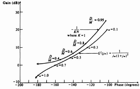
Figure 5.28 Compensation of a nonlinear system containing backlash, by reduction of the system gain.
The best approach for designing the phase-lead network is to use Eqs. (2.7) and (2.8), which are repeated here for solving for ωmax and φmax respectively:
To choose ωmax and φmax we analyze Figures 2.11 and 5.26. We will assume that the 1/α attenuation of the phase-lead network, shown in Figure 2.11, is compensated for by the control system's amplifier. In selecting ωmax and φmax we must take into account from Figure 2.11 that the gain characteristics of the phase-lead network increased with frequency, while the low-frequency portion (below 1/αT) will be unaffected (because the 1/α attenuation is compensated for). Therefore, it is advantageous to place ωmax at a relatively high frequency such as near the stable limit cycle at ω = 0.8139 and D/M = 0.1742, rather than at the frequency where the two curves have maximum phase overlap (at approximately ω = 0.7). Accordingly, we will add an additional phase of 29° at ωmax = 0.9. The result is αT = 1.9 and T = 0.65. For this system, a value of αT = 1.9 and T = 0.65 will eliminate the limit cycles, as illustrated in Figure 5.29. It is important to recognize, however, that this is not a unique solution. It is only one of many possible solutions, as can be noted from studying the gain-phase diagram.

Figure 5.29 Compensation of a nonlinear system containing backlash, by addition of a phase-lead network.
C. Introduction of Rate Feedback
Addition of rate feedback in parallel with position feedback can also be a very effective method for eliminating the oscillation. For this configuration, which is illustrated in Figure 5.30, the value of the system feedback element H(jω) is 1 + bjω which represents a pure zero. Therefore, the oscillation criterion for this configuration must be modified from that given by Eq. (5.81) to the following expression:
With rate feedback, the value of G(jω)H(jω) for the system being considered is given by

The best approach for selecting b is to recognize from Figure 5.30 that the rate feedback in parallel with position feedback results in a pure zero term (1 + bjω) as shown in Eq. (5.93). Therefore, it contributes a phase lead of tan−1 bω. Analysis of Figure 5.26 indicates that the maximum phase overlap is approximately 9° at ω = 0.7. We will design for an additional 7° for safety, and we can solve for b from
Therefore,
A value of b = 0.4 will eliminate the limit cycle, as is illustrated in Figure 5.31, and a relatively safe margin is achieved. At a value of b approximately equal to 0.25, the curves of G(jω)H(jω) and −1/N just clear each other.
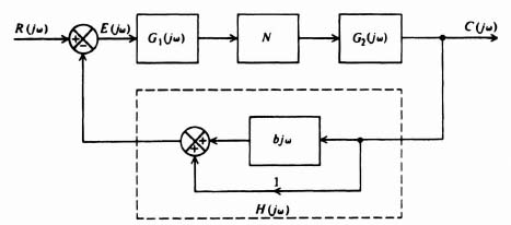
Figure 5.30 Nonlinear system containing rate and position feedback.
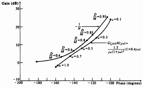
Figure 5.31 Compensation of a nonlinear system containing backlash, by the introduction of rate feedback.
A complete case study for the design of the positioning system of a tracking radar that uses conventional linear techniques and the describing function is presented jointly in Section 7.3. In this problem we show the separate linear and nonlinear considerations for the design of an actual control system, and their joint relationships.
5.11. DESCRIBING-FUNCTION ANALYSIS AND DESIGN USING MATLAB [29]
The use of MATLAB to analyze linear control sytems has been abundantly illustrated in previous chapters of this book. In this section, the application of MATLAB for analyzing the application of the describing functions for analysis and design is illustrated.
The AMCSTD Toolbox provides the following describing function utilities to supplement MATLAB and the Control System Toolbox:
- “deadzone” provides the normalized gain (N) for a given D/M and it also allows the refinement of a solution to the intersection of the dead-zone curve (−1/N) and a given transfer function for the linear portion of the control system. The AMCSTD Toolbox's command for this utility is

- “backlash” provides the gain (N) for any given D/M, and it also allows the refinement of a solution to the intersection of the backlash curve (−1/N) and a given transfer function for the linear portion of the control systems. The AMCSTD Toolbox's command for this utility is

- “relays” is a hysteresis utility with relay being a subset of its actual capability. It provides the gain (N) for any given set(s) of M, D, and H or H/D. It also allows the refinement of a solution to the intersection of the hysteresis curve (−1/N) and a given transfer equation for the lienar portion of the control system. The AMCSTD Toolbox's command for this utility is

The MathWorks has available a Nonlinear Control Design Toolbox for nonlinear control system analysis, which is illustrated in the AMCSTD Toolbox. The DEMO section of the AMCSTD Toolbox has many illustrations of the analysis of nonlinear systems using MATLAB.
A. Example 5.11-1
Let us now demonstrate the MATLAB program which provides the describing-function analysis illustrated in Figure 5.26. This is also illustrated in the DEMO example 5.2 in the AMCSTD Toolbox.
We will reconsider the nonlinear control system whose linear portion is represented by Eq. (5.84), which is repeated here,

and whose nonlinear portion is backlash. The MATLAB program to illustrate the backlash curves corresponding to Figures 5.15 and 5.16 is illustrated in the MATLAB program shown in Table 5.1, and is repeated in Figure 5.32. The MATLAB program to plot the describing function analysis shown in Figure 5.26 is given by the MATLAB program shown in Table 5.2, and is repeated in Figure 5.33.
Table 5.1. MATUB Program for Obtaining the Describing Function of Backlash
dm = linspace(.999,0);
n = back_lsh(dm);
subplot (211);
plot (dm, abs(n));
grid;
title('Backlash Amplitude'),
xlabel('D/M')
ylabel('IN(M)I'),
subplot (212);
plot(dm, angle(n)*180/pi);
grid;
title('Backlash Phase'),
xlabel('D/M'),
ylabel('Phase(Deg)')
|
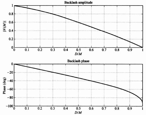
Figure 5.32 Describing-function for backlash.
Table 5.2. MATLAB Program for Obtaining the Describing Function Analysis for a Control System Containing Backlash and whose Linear Portion is Defined by Eq. 5.96
num = [0 1.5];
den = [1 1];
w = logspace(−1,0);
[mag,ph] = bode(num,den,w);
magdb=20*log10(mag);
dm=linspace(.95,0);
n = back_lsh(dm);
ninv = (0*n-1)./n;
xlabel('Phase(degrees)')
ylabel('Gain(dB)'),
w = [.1 .45 .6 1];
dm = [.9 .75 .6 .4 0];
grid;
title('Nonlinear Analysis for System Containing Backlash')
|
5.12. DIGITAL COMPUTER PROGRAMS FOR PERFORMING THE DESCRIBING-FUNCTION ANALYSIS
For those who do not have access to MATLAB, which has now become an industry standard (more or less), this book also provides another digital computer program for performing the describing function analysis. This approach for providing both MATLAB and other digital computer programs which are not dependent on COTS (commercial-off-the-shelf software) is used throughout this book.
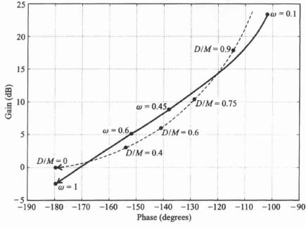
Figure 5.33 Describing-function analysis for a nonlinear control system containing backlash, whose linear portion is described by Eq. (5.84).
As shown in Sections 5.10 and 5.11 with the use of MATLAB, the digital computer is very useful for the construction of the describing function [25,38]. The computer can compute −1/N and, as indicated in Chapter 1, G(jω). This section illustrates the procedure used to analyze and compensate a practical nonlinear system containing backlash with the aid of a working digital computer program. It is based on the method illustrated in Sections 5.7 through 5.10. The Basic language will be used for this program [39,40].
Let us consider the system illustrated in Figure 5.5, where
and N corresponds to backlash. We know from Eq. (5.50) that

where
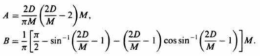
Note that the subscripts have been dropped from the A and B terms for simplicity. The coding symbols used are as follows:
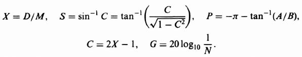
Figure 5.34a illustrates the logic flow diagram for developing the program for computing −1/N. Table 5.3 illustrates the actual program for computing −1/N. The reader should compare these two in order fully to understand the digital computer's program. Table 5.4 illustrates the computer run for calculating −1/N. Notice that is was necessary to compute additional values of 0.9 < D/M < 0.99 at the end of the computer run since it was found that a limit cycle existed in this region. Figure 5.34b illustrates the logic flow diagram for determining G(jω). In the coding G represents the gain of G(jω), P represents its phase and W represents ω. Table 5.5 illustrates the actual program for computing G(jω) and Table 5.6 illustrates the computer run for calculating G(jω).
The values for −1/N and G(jω) are illustrated on the gain-phase diagram in Figure 5.35. It indicates limit cycles at ω = 1.36, D/M = 0.41 (stable) and ω = 0.27, D/M = 0.945 (unstable). As illustrated previously in Section 5.10, this nonlinear system can be compensated by lowering the gain, by the addition of a phase-lead network or rate feedback. A similar analysis indicates that at K = 1.65, a phase-lead network given by

Table 5.3. Computer Program for Computing −1/N (Basic Program)
1 REM DESCRIBING FUNCTION FOR BACKLASH 10 PRINT “D/M”, “GAIN(DB)”, “PHASE(DEGREES)”, “N” 20 READ X1,X2,D 30 FOR X=X1 TO X2 STEP D 40 LET C=2*X-1 50 LET S=ATN(C/SQR(1-C↑2)) 60 LET A=1.27324*X* (X-1) 70 LET B=0.31831*(1.570796-S-C*COS(S)) 80 LET N=SQR(A↑2+B↑2) 90 LET G=20*0.43429448*LOG(1/N) 100 LET P=-180-57.29578*ATN(A/B) 110 PRINT X,G,P,N 120 NEXT X 130 DATA 0.05, 0.95, 0.05 140 END OK |

Figure 5.34 (a) Logic flow diagram for determination of −1/N.
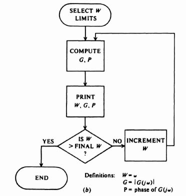
Figure 5.34 (b) Logic flow diagram for determination of G(jω).
Table 5.4. Results of Computer Analysis for −1/N

and rate feedback having a constant of 0.47 result in a 3-dB margin of safety. The system compensated with a phase-lead network and rate feedback is illustrated in Figure 5.35.
Table 5.5. Computer Program for Computing G(jω) (Basic Program)
10 PRINT “OMEGA”, “GAIN(DB)”, “PHASE(DEG)” 20 READ K 30 READ Wl,W2,D 40 FOR W=Wl TO W2 STEP D 50 LET G=4.342944S*LOG(K*K*(1+9*W*W)/(W*W*(1+4*W*W)↑2)) 60 LET P=-90+57.2957S*(ATN(3*W)-2*ATN(2*W)) 70 PRINT W,G,P 80 NEXT W 90 DATA 4,0.1,2.0,0.05 200 END |

Figure 5.35 Describing-function analysis based on computer program results.
Table 5.6. Results of Computer Analysis for G(jω)
5.13. PIECEWISE-LINEAR APPROXIMATIONS
Approximating any nonlinearity by means of piecewise-linear segmentation is a very useful tool for analysis. Each segment leads to a relatively simple linear differential equation which can be solved by conventional linear techniques. This method, which is not limited to quasilinear systems, has the advantage of yielding an exact solution for nonlinearities of any order, if the nonlinearity is itself piecewise linear or can be approximated by piecewise-linear segments. We illustrate its application by means of an example.
Let us consider saturation. Figure 5.36 illustrates a simple feedback control system containing an integrator and an amplifier which saturates. The amplifier gain is 5 over an input voltage range of ±1 V, for input voltages greater than this, the amplifier saturates. It is quite evident that two distinct linear operating regions for the amplifier exist. Each of these linear regions can be considered separately in a piecewise-linear manner in order to obtain the composite response of the system.
For the unsaturated region, the relationships depicting the system operation are
During saturation, Eqs. (5.100) and (5.102) are still valid. However, (5.101) changes to
Assuming zero initial conditions and a step input of 10V, the expression for the output during the saturated region of operation csat(t) is given by
The expression for the output during the unsaturated region is given by
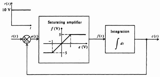
Figure 5.36 Feedback control system containing saturation.

The time t1 is the time at which the amplifier becomes unsaturated. When c = 9, e = 1, and t1 is 1.8 sec. Using conventional techniques, the solution to Eq. (5.106) is
The initial value for this region, cus(0), is the same as the final value of the saturated region, csat(1.8) = 9; this continuity of the output is imposed by the integrator. Therefore, the composite solution for this problem, obtained by a piecewise-linear analysis, is
The response of this system to a step input of 10V is sketched in Figure 5.37.
The piecewise-linear approach illustrated in the preceding problem can be extended to very complex nonlinearities. It is important to emphasize that the boundary conditions between linear regions are continuous whenever the transfer function following the nonlinearity is a proper rational function. The resulting differential equation for each segmented region is linear and can be easily solved by conventional linear techniques.
5.14. STATE-VARIABLE ANALYSIS: THE PHASE PLANE
A useful technique of applying the state-space approach to nonlinear systems is the phase-plane method [10, 11, 41]. It is a technique for analyzing the transient response of a nonlinear control system to an external input or for solving an initial-condition problem. The phase-plane method is limited to second-order systems. The variation of the displacement is plotted against velocity on a graph known as the phase-plane. A curve for a specific step input is known as a trajectory. A set of curves of displacment versus velocity of a specific system, which are repeated for several input values (or initial conditions) and are plotted on the same phase plane, is called a phase portrait.
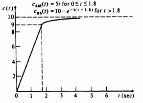
Figure 5.37 Step response of saturating system obtained from piecewise-linear analysis.
The starting point of a trajectory is the initial displacement, x(0), and velocity, (dx(0)/dt). The future path of the trajectory after it leaves its initial starting point represents the behavior of the control system for an input excitation. If the trajectory approaches infinity on the phase plane, the system is unstable. If the phase trajectory approaches the vicinity of the origin, however, the system is stable. If the trajectory circles the origin continuously in a closed curve after excitation, a sustained oscillation known as a limit cycle exists.
The phase-plane method is specifically concerned with the solution of second-order, nonlinear differential equations having the following general form:
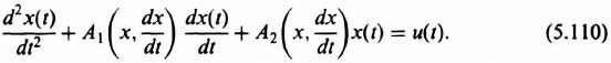
For our initial analysis, we will assume that the forcing function, u(t), equals zero and that the initial conditions, x(0) and (dx(0)/dt), represent the input to the system. Equation (5.110) immediately emphasizes some serious limitations of the phase-plane method. It is only useful for analyzing second-order systems. It is interesting to compare the limitations of the phase-plane method with those of the describing-function analysis, where the response to sinusoidal inputs of systems having any order could be determined. The phase-plane method could be extended to higher-order systems, but it is too impractical.*
The following section discusses the techniques which can be used for constructing the phase portrait from the differential equation of a system. Then we examine the properties and interpretation of the phase portrait. The procedure to be followed for applying the phase-plane approach to design problems, and a computer program for obtaining the phase plane are then presented.
5.15. CONSTRUCTION OF THE PHASE PORTRAIT
Four procedures that can be used to construct the phase portrait of a system are:
- direct solution of the differential equation;
- transformation of the second-order differential equation to a first-order equation;
- the method of isoclines;
- digital computer program.
The first two methods are analytical techniques; the third is graphical; the last is presented in Section 5.19. We shall describe these methods next, together with some illustrative examples.
A. Direct Solution of the Differential Equation
This is the most straightforward method for obtaining the phase portrait. It is usually the most useless method from a practical viewpoint, because we do not have to resort to the phase-plane representation for a solution if the differential equation is integrable. However, this method does provide an understanding of the situation.
The procedure is to solve the differential equation for the dependent variable x(t). The solution for x(t) is then differentiated in order to obtain the derivative of the dependent variable, dx(t)/dt. The dependent variable, time, is then eliminated between the two resulting equations. A single equation that relates x(t) and dx(t)/dt results, and can be used to plot the phase portrait directly. However, the approach has the disadvantage that it requires the solution of a nonlinear, second-order, differential equation.
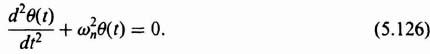
Let us illustrate the procedure in detail by first considering a simple linear system where a torque T(t) was applied to a body having a moment of inertia J, a twisting shaft having a stiffness factor K, and a damper having a damping factor B. Applying Newton's second law of motion to this system resulted in the following relationship:
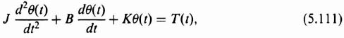
where θ(t) is the displacement. The differential equation is second order, and the phase-plane method is certainly applicable. Assuming that the system is unexcited, the resulting differential equation is given by
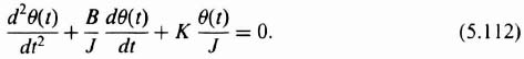
Equation (5.112) can be written in terms of damping ratio ζ and undamped natural frequency ωn, as follows.

where
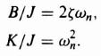
Before sketching the phase portrait, let us consider the simpler case of an undamped system where ζ = 0. For this situation, Eq. (5.113) reduces to

From elementary calculus, the solution to Eq. (5.114) is that of simple harmonic motion:
In order to obtain a relationship between θ(t) and dθ(t)/dt, we differentiate Eq. (5.115) and then eliminate time between the resulting equations, as follows:
Eliminating time between Eqs. (5.115) and (5.116), we obtain the expression
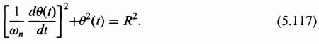
The phase portrait for this system can be drawn directly from Eq. (5.117). Observe that Eq. (5.117) describes a family of concentric circles in the (1/ωn)(dθ(t)/dt) versus θ(t) plane having a radius of R. Therefore, the phase portrait for this system (shown in Figure 5.38) is a family of concentric circles if a normalized ordinate axis is used. If the ordinate axis is not normalized, a family of ellipses results. Any set of initial conditions, such as points R1, R2, R3, and R4, specifies a particular circle. For t > 0, the motion is in the indicated direction. The origin is defined as a center, and is discussed further in Section 5.16.
Let us next sketch the phase portrait for the case where the damping ratio of this system is finite. The general solution for Eq. (5.113), when it is excited by a step input and has a set of initial conditions, was derived in Chapter 4‡ [see Eq. (4.45)‡]. The form of the solution for this system when it is unexcited by a step input and only has a set of initial conditions, θ(t0) and θ(t0), present is given by
Figure 5.38 Phase portrait for a second-order linear system having no damping. The origin is defined as a center.

Proceeding as in the previous example, the derivative of Eq. (5.118) is obtained:
The complexity of Eqs. (5.118) and (5.119) makes it quite difficult to eliminate time between them. Therefore we use an alternative approach. Equations (5.118) and (5.119) will be evaluated for several values of time to obtain the corresponding coordinates in a normalized phase plane. The result is plotted in Figure 5.39 for a damping ratio of 0.7. Notice that the phase portrait is a collection of noncrossing paths describing system behavior for all possible initial conditions. Because all the trajectories approach the origin of this system where u(t) = 0, the system is stable, as we would expect it to be. The origin is defined as a stable node, and is discussed further in Section 5.16.
The projection of a specific trajectory onto the abscissa gives the variation of θ(t) with time, and its projection onto the ordinate gives the variation of dθ(t)/dt with time. Time appears in the portrait implicitly as a parameter along all phase trajectories. We discuss its computation later in Section 5.16.
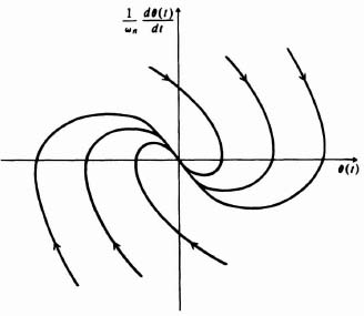
Figure 5.39 Phase portrait of a second-order linear system having damping. The origin is defined as a stable node.
Let us next illustrate the application of this method to a relatively simple nonlinear differential equation. We consider the problem of nonlinear friction which was discussed previously in Section 5.8. We first determine the phase portrait for Coulomb friction and then extend it to the case of stiction. Consider a system containing Coulomb friction ±Fc, the moment of inertia of the system being J and the spring constant K. The differential equation of the motion of the system is given by
Defining

the normalized equation of motion is
The phase portrait for Eq. (5.124) in the α(t) versus ![]() plane is the same as that for the linear, second-order system considered previously (see Figure 5.38). However, in the
plane is the same as that for the linear, second-order system considered previously (see Figure 5.38). However, in the ![]() versus c(t) plane, the phase portrait for Eq. (5.124) is quite different, and can be obtained by considering Eq. (5.124) in two parts: one for the upper half-plane where
versus c(t) plane, the phase portrait for Eq. (5.124) is quite different, and can be obtained by considering Eq. (5.124) in two parts: one for the upper half-plane where ![]() > 0, and the other for the lower half-plane, where
> 0, and the other for the lower half-plane, where ![]() < 0. A little thought shows that the phase portrait in the upper half-plane is a family of semi-circles, centered about c(t) = −γ, since c(t) is related to α(t) merely by a simple translation. In a similar manner, the phase portrait for the lower half-plane is a family of semicircles centered about c(t) = γ. Figure 5.40 illustrates the phase portrait.
< 0. A little thought shows that the phase portrait in the upper half-plane is a family of semi-circles, centered about c(t) = −γ, since c(t) is related to α(t) merely by a simple translation. In a similar manner, the phase portrait for the lower half-plane is a family of semicircles centered about c(t) = γ. Figure 5.40 illustrates the phase portrait.
It is interesting to observe from Figure 5.40 that as soon as the displacement has a value within the interval on the c(t) axis given by
all motion stops. This gives rise to the possibility of large, steady-state errors. For example, if the initial conditions are at point 1, the trajectory will be 1–2–3–4 and the system will not have any steady-state error. If the initial conditions are at point 5, however, the trajectory followed will be 5–6–7–8 and the system will have a steady-state error equal to γ.
We have already seen that dither is useful for eliminating the steady-state error due to Coulomb friction. Its effect on the steady-state error can easily be understood by studying the phase plane. For example, let us assume that a finite steady-state error exists corresponding to point 9 on Figure 5.40. With dither, the effect of a negative disturbance, segment 9–10, results in the system returning to point 11 on the c(t) axis, while a positive disturbance, segment 9–12, results in the system returning to point 13 on the c(t) axis. Because the projection 11–9 is greater than the projection 9–13, the system will tend to move towards the origin.

Figure 5.40 Phase portrait for a system containing Coulomb friction.
Before leaving this system, let us consider the required modification to the phase portrait in Figure 5.40 for stiction. Because stiction occurs only for zero velocity and is greater than Coulomb friction, its effect is to extend the termination line: ±γ to ±γs. These extended terminations are illustrated in Figure 5.40.
B. Transformation of the Second-Order Differential Equation to a First-Order Equation
If the differential equation of the system cannot be easily integrated, a new differential equation in terms of the phase variables may be formed, from which the phase portrait can be obtained directly. This method can best be illustrated by considering the linear, second-order, undamped system discussed previously, namely,
Using the dot notation, we have
Defining the state variables as
we have
Dividing Eq. (5.131) by Eq. (5.130), the following is obtained:
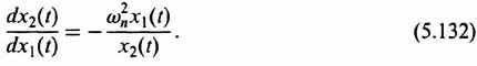
Equation (5.132) can be rewritten as
![]()
Integrating, we obtain
![]()
where C is an arbitrary constant easily determined from the initial conditions. Solving for x2(t), we obtain
![]()
In terms of the phase variable, this equation can be written as
The result of sketching various phase trajectories from Eq. (5.133) will be the phase portrait illustrated in Figure 5.38, where a normalized ordinate axis is used. The initial conditions determine the particular trajectory followed.
This techique can be easily extended to the systems whose phase portraits are illustrated in Figures 5.39 and 5.40. This method is by far the most useful analytic technique for obtaining the phase portrait of a system.
C. Method of Isoclines
The method of isoclines is a graphcial procedure for determining the phase portrait. It can be used even if the differential equation cannot be solved analytically. In practice, it is a very powerful method to use.
Isoclines are lines in the phase plane corresponding to constant slopes of the phase portrait. One starts with the differential equation in the form shown by Eq. (5.132). Here dx2/dx1(t), or d![]() (t)/dθ(t), corresponds to the slope of the trajectories that form the phase portrait. Numerical values are assigned for the slopes d
(t)/dθ(t), corresponds to the slope of the trajectories that form the phase portrait. Numerical values are assigned for the slopes d![]() /dθ(t), and Eq. (5.132) is used to find the corresponding points in the phase plane having those slopes. Once a set of isoclines is drawn, a trajectory may be drawn by starting at some point on an isocline and then proceeding to the next isocline along a straight line whose slope is the average of the slopes corresponding to the two isoclines. Because the procedure is a numerical approximation, closer spacing of the isoclines increases the accuracy of the resulting trajectory.
/dθ(t), and Eq. (5.132) is used to find the corresponding points in the phase plane having those slopes. Once a set of isoclines is drawn, a trajectory may be drawn by starting at some point on an isocline and then proceeding to the next isocline along a straight line whose slope is the average of the slopes corresponding to the two isoclines. Because the procedure is a numerical approximation, closer spacing of the isoclines increases the accuracy of the resulting trajectory.
Let us illustrate the application of the isocline method to the lienar, second-order, undamped, and damped sytems whose portraits are given in Figures 5.38 and 5.39, respectively. For the undamped case, the family of isoclines can be drawn from Eq. (5.132). However, in order to plot the phase portrait on a normalized plane [(1/ωn)![]() versus θ(t)], let
versus θ(t)], let
So we have
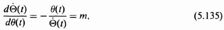
where m represents the slope of the trajectory.
Isoclines associated with slopes corresponding to Eq. (5.135) constitute a family of straight lines passing through the origin and are illustrated in Figure 5.41. Also shown is the construction of the phase trajectory starting with a point that lies on the isocline corresponding to a slope of −1.5. The motion of the trajectory drawn from point A on the −1.5 isocline, to the isocline whose slope is −2, has a slope in the phase plane that is the average of these two isoclines, or −1.75. This is indicated on Figure 5.41 as line segment AB. In addition, the following line segment, BC, whose slope is −2.5, is illustrated. The complete trajectory is shown dashed. It is obvious from this simple example that the accuracy of the isocline method depends on the number of isoclines drawn.
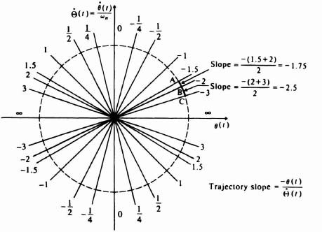
Figure 5.41 Construction of a phase trajectory for a linear, second-order, undamped system using the method of isoclines.
Let us next construct the phase portrait for the linear, second-order, damped system considered previously. From Eq. (5.112), the differential equation of the system is
Let us assume that ζ = 0.5 and using the dot notation, we have
Defining the state variables as
then we have
Dividing Eq. (5.141) by Eq. (5.140), we obtain the following:
Defining a normalized state variable

we can write Eq. (5.142) as follows:
or
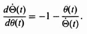
From this equation, the slope of the trajectories in the ![]() versus θ(t) plane is given by
versus θ(t) plane is given by

Isoclines associated with slopes corresponding to Eq. (5.144) constitute a family of straight lines passing through the origin in the phase plane. This is illustrated in Figure 5.42. The construction of the trajectory whose initial condition is a point which lies on the isocline corresponding to a slope of 2 is illustrated. The segment of the trajectory drawn from point A on the isocline whose slope is 2 to that whose slope is 1 would be a straight line whose slope is the average of 2 and 1, or 1.5. This is indicated in Figure 5.42 as line segment AB. In addition, the following line segment, BC, whose slope is 0.5, is illustrated. The remaining trajectory is shown dashed. As for the undamped system, the accuracy depends greatly on the number of isoclines drawn. Observe that the motion of the trajectory is in the clockwise direction about the origin because for positive x3(t), x1(t) must be increasing, and for negative x3(t), x1(t) must be decreasing [see Eq. (5.143)].
5.16. CHARACTERISTICS OF THE PHASE PORTRAIT
Several properties of the phase portrait need to be singled out; their correct interpretation is important for the intelligent analysis of nonlinear control systems. We begin by defining and illustrating the notion of singular points. Then we illustrate limit cycles and follow this by showing how to determine time from the phase portrait. The section concludes with examples of several interesting and representative phase portraits.
Figure 5.42 Construction of a phase trajectory for a linear, second-order, damped (ζ = 0.5) system using the method of isoclines.
A. Singular Points
Singular points are points of the phase plane where the system is in a state of equilibrium. At these points both velocity and acceleration of the system are zero. The origin is the only singular point in the phase portraits of the linear systems illustrated in Figures 5.38 and 5.39.
Consider the general second-order, nonlinear differential equation (5.110) which is unexcited from an external forcing function
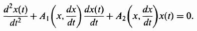
If this equation is written in the state-variable from, the singular points are defined as the points that make the quantities in Eqs. (5.145) and (5.146) equal to zero:

Here x(t) and y(t) are the state variables. The characteristics of singular points may vary greatly depending on the variations of the coefficients of the first-order differential equations given by Eqs. (5.145) and (5.146). The type of singular point may be found by means of a Taylor-series expansion of Eqs. (5.145) and (5.146) in the vicinity of the singular point. Assuming that the singularity occurs at x(t) = A and y(t) = B, the result of expanding P(x, y) and Q(x, y) about these points is

We assume that the character of the singular points is determined entirely by the coefficients of the linear terms only: A1, A2, B1, and B2. This is certainly reasonable if a sufficiently small region is chosen in the vicinity of the singularity. What we have done is to characterize the system by its linear part in the vicinity of the singular point. Therefore, Eqs. (5.147) and (5.148) reduce to

We further simplify the problem by assuming that the singularity occurs at the origin. Therefore A and B are both zero. Equations (5.149) and (5.150) reduce to the form
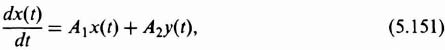
We have not lost any generality in using this assumption, because the same result can always be obtained merely by changing the variables as follows:
The characteristics of the singular point can be determined by eliminating one of the two variables of Eqs. (5.151) and (5.152) and studying the resulting characteristic equation. Using the Laplace transform, the result is
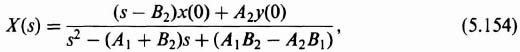
and the characteristic equation is given by
Assuming real coefficients, six different characteristic sets of roots of Eq. (5.155) are possible. These sets of roots result in singular points which can be classified as belonging to one of four types.
1. Node. A node is a point in the phase plane consisting of a family of trajectories which directly converge and approach it (stable node) or radiate from it (unstable node). A stable node occurs when the roots are both real and both lie in the left half of the s-plane. An unstable node occurs when the roots are both real and both lie in the right half of the s-plane. Figure 5.39 illustrates a stable node and Figure 5.43 an unstable node.
2. Focus. A focus is a point in the phase plane consisting of a family of spiral trajectories which either converge on the point (stable focus) or diverge from it (unstable focus). A stable focus occurs when the roots are complex conjugate and lie in the left half of the s-plane. An unstable focus occurs when the roots are complex conjugate and lie in the right half-plane. The origin of the phase portrait in Figure 5.44 is a stable focus. Figure 5.45 illustrates an unstable focus.
3. Center. A center is a point in the phase plane consisting of a family of closed curves encircling it. This occurs when the roots are complex conjugate and lie on the jω axis. The origin of the phase portrait in Figure 5.38 is a center.
4. Saddle Point. A saddle point is a point in the phase plane that is characterized by the phase portrait illustrated in Figure 5.46. This occurs when the roots are real, with one in the right half-plane and the other in the left half-plane. Except for the case where the numerator of Eq. (5.154) contains a zero which exactly cancels the zero of the denominator lying in the right half-plane, this type of singularity always represents an unstable situation.
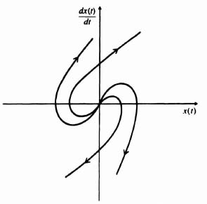
Figure 5.43 Phase portrait of an unstable node.

Figure 5.44 Phase portrait of a stable focus.

Figure 5.45 Phase portrait of an unstable focus.
B. Limit Cycles
Limit cycles are defined as isolated closed paths of the phase portrait. The location and determination of the type of limit cycle, together with the singular points which exist in the phase plane, offer a complete description of the behavior of a nonlinear second-order system.
A limit cycle can be stable or unstable, depending on whether the paths in the neighborhood of the limit cycle converge toward it or diverge away from it. They can result from either soft or hard self-excitation. These situations can be portrayed on the phase plane. Figure 5.47 illustrates a system with a soft-excitation. Physically, this phase portrait may represent a system which has excessive gain for small signals and the output builds up in an unstable manner. With large signals the output also approaches the stable limit cycle from the outside as shown in Figure 5.47. A stable limit cycles exists between these two conditions and a sustained oscillation occurs. Figure 5.48 illustrates a system where a hard-self-excitation exists. The generation of an oscillation depends on the initial conditions. For example, let us assume that the initial state is at the stable node. For hard self-excitation to occur, a very large disturbance is required to change the state of the system to a region outside the unstable limit cycle. If this disturbance is sufficient for the operating point of the system to reach the stable limit cycle, a steady oscillation occurs.
Observe that all of the trajectories in Figures 5.38 through 5.48 are perpendicular to the x axis because the isocline slopes there are infinity (see Figure 5.41).
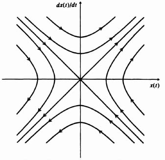
Figure 5.46 Phase portrait of a saddle point.
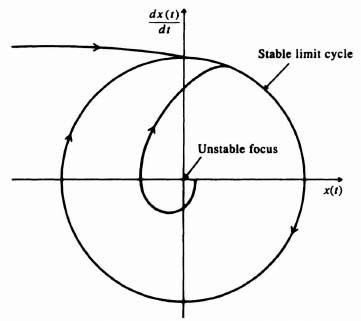
Figure 5.47 Phase portrait of a soft self-excitation.

Figure 5.48 Phase portrait of hard self-excitation.
C. Determination of Time from the Phase Plane
Although we cannot solve for x(t) and dx(t)/dt as functions of time directly, it is possible to obtain time from the phase portrait. The variation of time can be easily found from the equation.
Solving for t, we obtain the relationship

Equation (5.157) shows that if the phase portrait is replotted with 1/y(t) or (dx(t)/dt)−1 as the ordinate and x(t) as the abscissa, the area under the resulting curve represents time. This area can be evaluated with a planimeter, crudely by approximation using a series of rectangles, or with a computer if we know mathematical expressions for the segments of the phase trajectory. If we know mathematical expressions for the segments of the phase trajectory, in a piecewise-linear manner, then we can also find the time directly by integrating Eq. (5.157).
Let us use the phase trajectory labeled ABCDEF on the phase portrait of Figure 5.44 to illustrate the determination of time graphically. We assume that ωn = 1. Our first problem is to determine the time it takes for the motion to go from A to C. Figure 5.49 represents a plot of [dθ(t)/dt]−1 versus θ(t) for the interval ABC. Using a series of rectangles for area summation, we find that the time is approximately equal to 1.12 sec. If we attempt to find the time it takes for the trajectory to pass from C to E, we run into a problem, because dθ(t)/dt equals zero at point D and the reciprocal phase-plane plot goes to infinity. This certainly is not the true situation, and we must resort to an approximation in the vicinity of point D. The most practical approximation is to find the time it takes to go from point C to a small finite distance on the phase trajectory before point D, D(−), and then the time it takes to go from a small finite distance past point D, D(+), to point E. This technique is illustrated in Figure 5.50. Using the rectangular area summation technique, we find that it takes approximately 2.18 sec to go from point C to point E. Therefore, the total time it takes to traverse the segment ABCDE is approximately 3.3 sec.
An interesting observation to question is why does it take a longer time for the trajectory to go along segment CDE (2.18 sec) than segment ABC (1.12 sec), although the trajectory segment CDE is smaller than the trajectory segment ABC (see Figure 5.44)? The answer is that the control system is slowing down as the trajectory follows A to B to C to D to E to F, and ultimately comes to rest at point F. Therefore, it takes longer to pass from C to D to E than it does from A to B to C.
Figure 5.49 Finding time from a reciprocal phase-plane plot.

Figure 5.50 Approximating time from a reciprocal phase-plane plot when velocity passes through zero.
As was pointed out earlier, the time can be determined by integrating Eq. (5.157) directly if we know mathematical expressions for the segments of the phase trajectory (in a piecewise-linear manner), rather than using a series of rectangles for area summation as was done in this problem.
D. Representative Phase Portraits
In order to develop a great facility for intelligently interpreting phase portraits, we next present additional representative phase portraits. These, with the portraits already discussed, should provide a good facility for interpreting phase portraits. Specifically, we consider the phase portraits of undamped, second-order control systems that have the nonlinear characteristics of rate and position limiting. We compare the results with the portrait illustrated in Figure 5.41.
1. Rate Limiting of an Undamped, Second-Order System. Consider the linear, undamped, second-order system whose phase trajectory was illustrated in Figure 5.41. We shall change this linear system to a nonlinear one by adding a governor to the servomotor driving the load so that the maximum rate is limited. The resulting phase portrait is illustrated in Figure 5.51. If the initial conditions are such that the resulting phase trajectory lies anywhere within the dashed trajectory, the system will oscillate as the undamped linear system did, as shown in Figure 5.41. However, if the initial conditions are such that they lie outside the dashed trajectory of Figure 5.51, the output rate is limited to the maximum value allowed by the governor, as shown in Figure 5.51 by the dashed trajectory. Thereafter the system will oscillate indefinitely following the dashed trajectory.
2. Position Limiting of an Undamped, Second-Order System. Next consider the linear, undamped, second-order system that is made nonlinear by adding limit stops to the output shaft, so that the maximum positions are limited. The resulting phase portrait is given in Figure 5.52. The interpretations of this phase portrait is analogous to that of Figure 5.51, except that it is shifted by 90°.
5.17. PHASE PLANE FOR SYSTEMS CONTAINING EXTERNAL FORCING FUNCTIONS
In the preceding analysis of the phase plane, we have always assumed that the extenral forcing functions were zero, and that the system excitation came from the initial conditions. We will reconsider the nonlinear differential equation (5.110) when there is an external forcing function u(t).
To illustrate the modification to our previous analysis, let us consider the linear second-order system illustrated in Figure 5.53. We want to find the phase trajectory of the system in the c(t) vs. ![]() phase plane upon the application of a unit step, r(t) = U(t). We will assume that the system's initial conditions are
phase plane upon the application of a unit step, r(t) = U(t). We will assume that the system's initial conditions are ![]() , and that the system is underdamped. This results in the characteristic exponentially damped sinusoid response illustrated in Figure B.4. Figure 5.54a illustrates the corresponding phase trajectory for this case. Observe from this figure that the value of the maximum overshoot of the system, c(t)max [see Eq. (B.32)] can be found from the phase trajectory. Figure 5.54b illustrates the phase trajectory when the system is critically damped.
, and that the system is underdamped. This results in the characteristic exponentially damped sinusoid response illustrated in Figure B.4. Figure 5.54a illustrates the corresponding phase trajectory for this case. Observe from this figure that the value of the maximum overshoot of the system, c(t)max [see Eq. (B.32)] can be found from the phase trajectory. Figure 5.54b illustrates the phase trajectory when the system is critically damped.
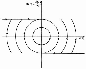
Figure 5.51 Phase portrait of a second-order, undamped system having rate limiting.
Figure 5.52 Phase portrait of a second-order, undamped system having position limiting.

Figure 5.53 A linear, second-order system.

Figure 5.54 Phase plane for the output trajectory of a linear, second-order system having a step input for the cases when it is (a) underdamped and (b) overdamped.
We know from Figure C.4 the shape of the error's transient for a linear second-order system to a step input. How would the error's transient appear as a phase trajectory in the e(t) vs. ![]() phase plane? We will first assume that the system is underdamped, and then we will assume critical damping. Figure 5.55a illustrates the corresponding phase trajectory for the underdamped case and Figure 5.55b illustrates the phase trajectory for the critical damping case.
phase plane? We will first assume that the system is underdamped, and then we will assume critical damping. Figure 5.55a illustrates the corresponding phase trajectory for the underdamped case and Figure 5.55b illustrates the phase trajectory for the critical damping case.
As another interesting example, suppose that the input to the system of Figure 5.53 has an input that is a ramp, r(t) = Vt, and the system is assumed to be under-damped. We wish to find the phase trajectory of the system in the e(t) vs ![]() phase plane. From Figure 5.53, we find that
phase plane. From Figure 5.53, we find that

Therefore, in the time domain,
Because we know that
substituting Eq. (5.160) into Eq. (5.159), we obtain
![]()
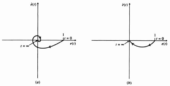
Figure 5.55 Phase plane for the error trajectory of a linear, second-order system having a unit step input for the case when it is (a) underdamped and (b) overdamped.
Because ![]() is given as
is given as
then
Substituting Eqs. (5.162) and (5.163) into Eq. (5.161),
Since ![]() in the steady state, then a singularity at
in the steady state, then a singularity at
exists, and the phase trajectory starts at its initial condition of ![]() and terminates at its singularity defined by Eq. (5.165) as illustrated in Figure 5.56.
and terminates at its singularity defined by Eq. (5.165) as illustrated in Figure 5.56.
5.18. DESIGN OF NONLINEAR FEEDBACK CONTROL SYSTEMS USING THE STATE-VARIABLE PHASE-PLANE METHOD
This section illustrates the design of a nonlinear feedback control system using the phase-plane method [41]. We use the analytic tools developed in Sections 5.14–5.17 to demonstrate the procedure to follow when designing a nonlinear system. Specifically, we consider an on-off control system. The primary function of this example is to use the transient response of the system as a guide for choosing the parameters. One of our main objectives will be to determine the existence of limit cycles as the parameters are varied. We will not, however, be able to obtain the margin of stability for the system from the phase plane. The following analysis should be compared with that obtained using the describing function for design in Section 5.10.
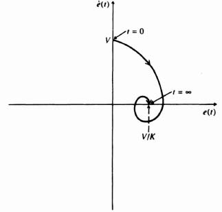
Figure 5.56 Phase plane for the error trajectory of a linear, second-order system having a unit ramp input Vt for an underdamped system.
Let us consider the on-off control system illustrated in Figure 5.57. It has a two-position contactor which applies a corrective signal having the proper phase for control action. The problem is to determine a good polarity combination of the variable position feedback constant a and the variable velocity feedback constant b for stability and acceptable transient performance. We assume that the input r(t) is zero and that the forcing function generated by the contactor is unity; therefore the general form of the differential equation for this system is given by

where 0 < ζ < 1. The sign of the unit forcing function is given by the sign of ac + b(dc/dt). Assuming that ζ = 0.5 and ωn = 1, the equation reduces to

Figure 5.57 On-off control system having variable position and velocity feedback.
Specifically, we shall determine the transient response of this system for the following polarity combinations of a and b:

In general the phase portrait for any of these cases may be obtained in a similar manner. We draw heavily on the results of our studies of singular points (see Section 5.16) in drawing the various phase portraits. The basic relation analyzed in our discussion of singular points was Eq. (5.110):

If we are considering an underdamped, linear second-order system which is excited only by its initial conditions, we know that the differential equation (5.113) results in a phase portrait similar to that in Figure 5.39, where the origin acts as a stable node. In the case of an on-off system, however, we find that it is represented by a differential equation which is given by Eq. (5.167). The right-hand side of this equation can be thought of as either a unit positive or negative forcing function. The phase portrait of a system having a unit positive forcing function will have spirals that converge towards a stable focus at x = 1, dc/dt = 0. This was discussed in Section 5.17, and illustrated in Figure 5.54. The phase portrait of a system having a unit negative forcing function will have spirals that converge towards a stable focus at c = −1, dc/dt = 0. The on-off system we are considering actually has two stable foci because of the action of the two-position contactor. A switching line, defined by
separates the regions where the phase trajectory spirals towards c = 1, dc/dt = 0 or c = −1, dc/dt = 0. Using this general approach, which is valid for all four cases, stability and the transient response can be readily determined.
Case A. a > 0, b > 0. The switching line is a straight line given by the following relationship:
It passes through the origin and lies in the second and fourth quadrants. The sign of ac + b(dc/dt) is positive in the region to the right of it and negative to the left of it. The phase portrait for this system, which is given in Figure 5.58, can be constructed using the method of isoclines or by transforming the second-order differential equation to a first-order equation or by use of a digital computer (see Section 5.19). Observe that three trajectories are possible, depending on the initial conditions. Two represent convergent motion where the phase portrait terminates on the foci at −1 or 1, depending on the final switching input. The third possible trajectory represents a limit cycle.
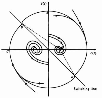
Figure 5.58 Phase portrait for an on-off control system where a > 0 and b > 0.
Any initial condition occurring beyond the limit cycle or very close to it in the enclosed area will eventually result in the trajectory reaching some part of the limit cycle, ABCDA. For a limit cycle to occur, the distance DE from the switching line to the corresponding focus must be greater than the distance BE, which represents the distance from the subsequent crossing of the line to the focus. This must be true with respect to the other focus as well. Trajectories that start sufficiently inside the limit cycle will spiral into one of the foci.
Case B. a > 0, b < 0. The switching line is a straight line given by

It passes through the origin and lies in the first and third quadrants. In a manner similar to the first case, we can show the phase portrait to be as shown in Figure 5.59. Observe that any set of initial conditions which results in a trajectory intersecting the switching line inside the interval AB results in a motion spiraling towards one of the two stable foci. However, if the intersection occurs outside the interval AB, the trajectory theoretically ends on the switching line. Figure 5.59 indicates these points by C and D. Points E and F represents points of tangency with the switching lines for limiting trajectories. In reality, however, the system cannot just end at these points. This inconsistency is resolved by the fact that switching action of a contactor always has a certain time lag due to its dynamics. Therefore, when a solution reaches the switching line it actually proceeds for some small distance past it, before there is a change of sign in the forcing function. This results in a zigzag action along the switching line. Eventually, the trajectory spirals into one of the focis as shown in Figure 5.59. Physically, this is audible as a “chattering” of the contactor.

Figure 5.59 Phase portrait for an on-off control system where a > 0, b < 0.
Case C. a < 0, b > 0. The switching line has the same form as that of case B. The phase portrait is given in Figure 5.60. For this case a stable limit of cycle always prevails. Regardless of the initial conditions, the final solution always winds up as a stable limit cycle.
Case D. a < 0, b < 0. The switching line has the same form as that of case A. The phase portrait, given in Figure 5.61, shows that no periodic solution exists. The solutions tend to end on the switching line. Because of the time lag of the relay, however, the trajectory zigzags towards the origin of the phase plane. The system finally oscillates at very high frequency and small amplitude around the origin.
It is interesting to observe that of the four cases considered, the control-system engineer would prefer the phase portrait of case D, the only configuration which resulted in a stable equilibrium state occurring around the origin. [Remember that r(t) = 0 and, therefore, c(t) = 0 in the steady-state as t approaches infinity.] However, we would have to tolerate some chattering around the origin with this linear switching system. To eliminate the chattering, one would have to use nonlinear switching techniques.

Figure 5.60 Phase portrait for an on-off control system where a < 0, b > 0.
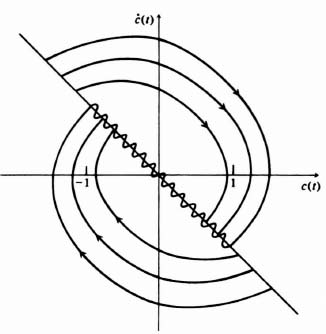
Figure 5.61 Phase portrait for an on-off control system where a < 0, b < 0.
5.19. DIGITAL COMPUTER PROGRAM FOR OBTAINING THE PHASE PLANE
This section presents a working program for obtaining a phase trajectory on the phase plane, and it applies the program to a practical system. The Fortran language will be used for the program.
Let us consider the linear, second-order system illustrated in Figure 5.62. It is desired to determine the phase trajectory of this system for the following set of initial conditions:
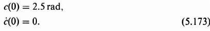
It is assumed in this problem that the system does not have any external forcing function. The program used will determine the phase trajectory using the method of isoclines.
The isocline for this system is obtained as follows. The closed-loop transfer function of the system in Figure 5.62 is given by
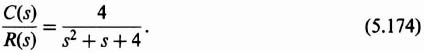
In the time domain, the differential equation describing this equation is given by
Because the system does not have any external forcing function, r(t) = 0, and Eq. (5.175) reduces to
Defining the state variables as
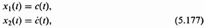
we obtain the following state equations to represent this system:
Dividing Eq. (5.179) by (5.178), we obtain the following:
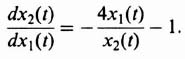

Figure 5.62 Linear, second-order system whose phase trajectory is to be obtained for initial conditions of c(0) = 2.5 rad and ![]() = 0.
= 0.
Simplifying this equation, we obtain the following:
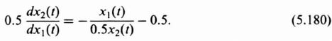
Defining a normalized state variable
we can rewrite Eq. (5.180) as follows:
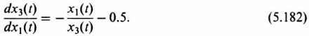
Defining
Eq. (5.182) can be rewritten as

Therefore, the slope of the trajectories in the ![]() vs c(t) plane is given by
vs c(t) plane is given by
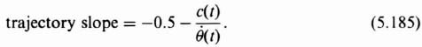
Figure 5.63 illustrates the logic flow diagram for developing the program for computing the isocline lines and the phase trajectory. Table 5.7 illustrates the actual Fortran program for determining the isoclines and the phase trajectory. Table 5.8 illustrates the program output for determining the phase plane for the system of Figure 5.62 with the initial conditions given by Eq. (5.173). A plot of the results is given in Figure 5.64. The plot also compares the phase trajectory obtained using the method of isoclines with the theoretically obtained phase trajectory. An analysis of the resulting phase trajectory in the phase plane of Figure 5.64 indicates that the resulting trajectory has a stable node at the origin, and it is similar to the phase plane of Figure 5.42.
5.20. LIAPUNOV'S STABIUTY CRITERIA
A. M. Liapunov [2] developed a fundamental method of determining the stability of a dynamic system based on generalization of energy considerations. This section presents the first and second methods of Liapunov and illustrates their application to nonlinear control systems [3,37].
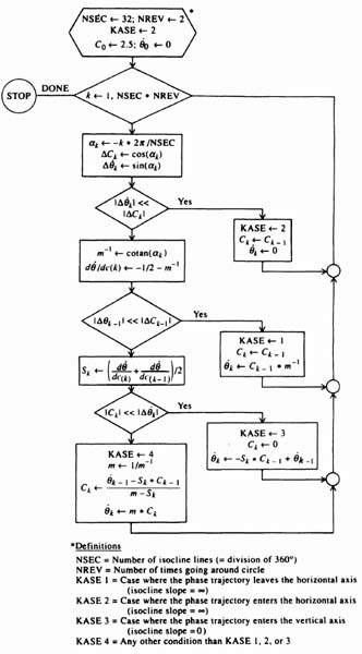
Figure 5.63 Logic flow diagram for phase-plane analysis.
Table 5.7. Computer Program for Phase-Plane Analysis (Fortran Program)
data NSEC/32/.NREV/2/,C1/2.5/,DTH1/0.0/,KASE/2/,PI/3.141593/
       print55, C1, DTH1
       do 100 K=1, NSEC*NREV
         ANGLE=-K*2*PI/NSEC
         YDEL=sin(ANGLE)
         XDEL=cos(ANGLE)
c      see if 1/SLOPE → infinity (occurs at 0 or 180 degrees)
       if (ABS(XDEL).ge.IE-35) then
         if (ABS(YDEL/XDEL).le.1E-5) then
           KASE=2
           C=C1
           DTH=0
           goto80
         endif
       endif
c      otherwise, it's OK to compute 1/SLOPE
       SLPINV=cotan(ANGLE)
       DDTH=-0.5-SLPINV
c      see if 1/SLOPE → infinity on the previous loop iteration
       if (KASE.eq.2) then
          KASE=1
          C=C1
          DTH=C/SLPINV
       else
c        otherwise, calculate isocline intersection point
         S=(DDTH+DDTH1)/2
c        see if SLOPE → infinity occurs at 90 or 270 degrees)
         if (ABS(YDEL).ge.1E-35) then
           if (ABS(XDEL/YDEL).le.1E-5) then
             KASE=3
             C=0
             DTH=-S*C1+DTH1
             goto80
           endif
         end if
c        otherwise, both SLOPE & 1/SLOPE are finite → solve 2 equations
         KASE=4
         SLOPE =1/SLPINV
         C=(DTH1-S*C1)/(SLOPE-S)
         DTH=SLOPE *C
       end if
80     continue @ come here to escape more testing
       print60, C, DTH, DDTH, DDTH1, S, KASE
       C1=C
       DTH1=DTH
       DDTH1=DDTH
100  continue
     print65
 55  format(7x, 'C   THETA-DOT   I.S.1  I.S.2  AVG.SLOPE',
     $' *CASE'/7x,'= ========    =====   ==== ',
     $ ========  ===='//2e12.4, '---> (INITIAL CONDITIONS)')
 60  format(5e12.4, I5)
 65  format(/' *NOTE: CASE=1 or 2 --> ISOCLINE SLOPES 1 OR 2 DIVERGE'/
     $      '         CASE=3 OR 4 --> ISOCLINE SLOPES VALID')
      end
|
Table 5.8. Program Output for Phase Plane of System in Figure 5.62

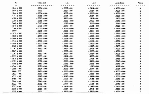
*NOTE: CASE = 1 or 2 → ISOCLINE SLOPES 1 OR 2 DIVERGE
CASE = 3 OR 4 → ISOCLINE SLOPES VALID
Figure 5.64 Phase trajectory for system of Figure 5.62.
A. Liapunov's First Method
Liapunov divided the general problem of analyzing the stability of nonlinear control systems into two classes. The first class consists of all those methods in which the differential equation of the system can be solved. System stability or instability is determined from this solution. This approach, which is known as Liapunov's first method, does not say anything of particular importance concerning the solution of the nonlinear differential equations. However, Liapunov did point out in his first method that the solution may be obtained in the form of a series from which stability can be determined using his second method. In addition, he proved that approximate solutions of nonlinear differential equations often yield useful stability information.
In order to illustrate Liapunov's first method, let us assume that the nonlinearity is single valued (has no hysteresis present) and has derivatives of every order in the vicinity of a point A. The nonlinear function, u = f(x), can be expanded into a Taylor series as follows:
Note that the first two terms of the series represent the linear approximation about the operating point of the actual nonlinearity. Liapunov proved that if the real parts of the roots of the characteristic equation corresponding to the differential equation of the linear approximation are different from zero, the equations of the linear approximation always give a correct answer to the question of staiblity of a nonlinear system [3,37]. This theorem means that we can use a linear approximation of the nonlinear equation and determine stability from it. If the roots of the linearized characteristic equation are negative, the motion is stable about the point in question. However, if any of the real parts of the roots of the characteristic equation of the linear approximation are positive, the motion is unstable about the operating point. In the special case of roots of the linearized characteristic equation having zero real parts, no conclusion may be drawn.
To illustrate the application of Liapunov's first method, consider the Van der Pol equation which describes the voltage buildup of an oscillator,
where
![]()
The equilibrium point of this system is determined when the velocity and acceleration are zero. Then,

In order to determine behavior in the area of the equilibrium point V, let
where
![]()
Substituting Eq. (5.190) into Eq. (5.187) we obtain the following expression:
The linear approximation to this equation is given by
The characteristic equation is given by
Applying the Routh–Hurwitz stability criterion, we find that, for stability,
Equation (5.194) states that when u < 0, the system is stable for all |V| < 1. Liapunov's first method is not applicable when V = 1, because this condition results in zero real parts for the roots of the characteristic equation.
It is important to emphasize that Liapunov's first method determines stability in the immediate vicinity of the equilibrium point.
B. Liapunov's Second Method
This determines stability without actually having to solve the differential equation. In this method a function of the state variables having special properties is formed that can be compared to the sum of the kinetic and potential energy, and the derivative of the function with respect to time is taken. If this derivative is negative along the trajectories of the system, it can be shown that the system is asymptotically stable. The remainder of this section is devoted to the details and application of the method.
We introduce Liapunov's second method by first considering a linear system. Reconsider the simple mass-spring-damper mechanical system considered in Section 5.2. It was shown there that this system can be represented by the following differential equation:
Assume that M = B = K = 1 and that f(t) = 0. Then we have
Defining the state variables as
the system can be described by the following two first-order differential equations:
This simple linear system can easily be solved. Assuming the initial conditions are
then we obtain the following solutions:
Equations (5.203) and (5.204) are plotted in the time domain in Figure 5.65, and in the phase plane in Figure 5.66. These two figures completely determine the dynamics and stability of this simple mechanical system. The system is stable and the states x1(t) and x2(t) behave as indicated.
Now, let us look at this simple system from the viewpoint of energy. The total stored energy is given by

Figure 5.65 Time-domain response of a simple mechanical system.
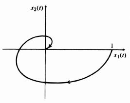
Figure 5.66 Phase trajectory of a simple mechanical system.
Because K = M = 1 in our simple example,
This total energy is dissipated as heat in the damper at the rate of
Because B = 1, we obtain
Equation (5.206) determines the loci of constant stored energy in the x1(t)x2(t) plane. Clearly they are circular for this simple example. Another important observation from Eq. (5.208) is that the energy rate is always negative and, therefore, these circles must get smaller and smaller with time. Figure 5.67 illustrates this characteristic in the phase plane. For this simple example, we can determine the time variation of V(t) and ![]() explicitly by substituting Eqs. (5.203) and (5.204) into Eqs. (5.206) and (5.208). The results are as follows:
explicitly by substituting Eqs. (5.203) and (5.204) into Eqs. (5.206) and (5.208). The results are as follows:
Figure 5.68 illustrates the time variation of V(t) and ![]() . Comparing Figures 5.67 and 5.68, we conclude that the total stsored energy approaches zero as time approaches infinity. This implies that the system is asymptotically stable. By this is meant that the state will return to the origin from any point x(t) within a region R enclosing the origin. Asymptotic stability is the type of stability preferred by control engineers because it excludes a stable limit cycle.
. Comparing Figures 5.67 and 5.68, we conclude that the total stsored energy approaches zero as time approaches infinity. This implies that the system is asymptotically stable. By this is meant that the state will return to the origin from any point x(t) within a region R enclosing the origin. Asymptotic stability is the type of stability preferred by control engineers because it excludes a stable limit cycle.
The stability of nonlinear control systems depends on the particular state space in which the state vector ranges in addition to the type and magnitude of the input. Therefore, the stability of nonlinear control systems can also be classified on a regional basis as follows [6, 16]:
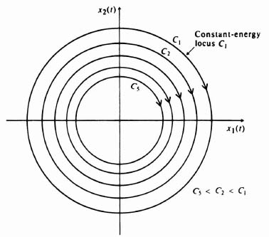
Figure 5.67 Constant-energy loci on the phase plane illustrating a decrease of energy with time.

Figure 5.68 Variation of energy and energy rate with time.
- local stability, or stability in the small,
- finite stability,
- global stability, or stability in the large.
A nonlinear control system is denoted as being locally stable if it remains within an infinitesimal region about a singular point when subjected to a small perturbation. Finite stability refers to a system which returns to a singular point from any point x(t) within a region R of finite dimensions surrounding it. The system is said to be globally stable if the region R inclues the entire finite state space. Stability of either the local, finite, or global variety does not exclude limit cycles, but rather only excludes the possibility of the state point tending to travel to infinity. If the state point approaches the singularity as time approaches infinity, for any initial conditions within the region under consideration, then the system is described as being asymptotically stable. Asymptotic stability excludes a stable limit cycle as a possible dynamic equilibrium condition. The strongest possible condition that can be placed on a nonlinear control system, with parameters that do not vary with time, is global asymptotic stability.*
The formal definitions of positive definiteness of a scalar function V(x) and similar functions are as follows.
1. Positive Definiteness of Scalar Functions. The scalar function V(x) is positive definite in a region which includes the origin of the state space if V(x) > 0 for all nonzero states x in the region, and V(0) = 0. An example of a positive definite scalar function is
2. Negative Definiteness of Scalar Functions. The scalar function V(x) is negative definite if −V(x) is positive definite. An example of a negative definite scalar function is
3. Indefiniteness of Scalar Functions. The scalar function V(x) is indefinite in a region if it contains both positive and negative values. An example of an indefinite function is
4. Quadratic Form of Scalar Function. The following quadratic form of the scalar function is also used very frequently in the analysis of the second method of Liapunov:
where x is a real vector and A is a real symmetric matrix.
The positive definiteness of the quadratic form of V(x) is determined using Sylvester's criterion, which states that the necessary and sufficient conditions for the quadratic form of V(x) to be positive definite are that all of the successive principal minors of the symmetric matrix A be positive. For example, let us assume that A is given by:
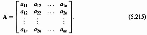
Therefore, the necessary and sufficient condition are that all the successive principal minors of A are positive as follows
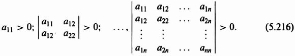
As an example to illustrate the application of the quadratic form and Sylvester's criterion to test the positive definiteness of the energy function V(x), consider the following scalar function V(x):
Applying the quadratic form of V(x), we can express this in terms of the unknown elements of A as follows:
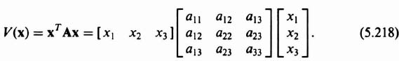
We can multiply the matrices xT, A, and x and obtain the following in terms of the unknown elements of A as follows:

Setting like coefficients of Eqs. (5.217) and (5.219) equal to each other, we find the values of the elements of the A matrix. The resulting A matrix is as follows:
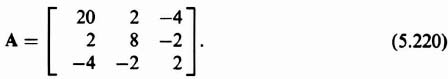
Applying Sylvester's criterion we find that

In conclusion, since all of the successive principal minors of the matrix A are positive, then V(x) is a positive definite scalar function.
A major factor in this analysis has been the choice of the energy function V(t),
This function has two very interesting properties. First it is positive for all nonzero values of x1(t) and x2(t). Secondly, it equals zero when x1(t) = x2(t) = 0. A scalar function having these properties is called a positive-definite function. By adding V(t) as a third dimension to the x1(t)x2(t) plane, the positive-definite function V(x1, x2) appears as a cup-shaped three-dimensional surface as illustrated in Figure 5.69.
Liapunov's stability theorem can now be summarized for n-dimensional state space. A dynamic system of nth order is asymptotically stable if a positive-definite function V(t) is found whose derivative with respect to time is negative along the trajectories of the system. In practice, it is fairly easy to find a function which is positive definite, but usually it is very hard to find a function where, in addition, ![]() < 0 along the trajectories.
< 0 along the trajectories.
A justification of Liaponov's second method can best be presented by considering the phase plane of Figure 5.70. Contours of constant V(t) are shown by the curves of C1, C2, and C3. Assume that the phase trajectory of this second-order system, whose initial state is the point p, is described by the following state equations:
The positive-definite function V(t) is assumed to be given by
where a and b are unknown coefficients. The quantity V(t) is permitted to take on successively larger constant values,
Figure 5.69 A positive-definite function.
Figure 5.70 Justification of Liapunov's stability criterion.
Therefore, Eq. (5.225) results in a set of equations:
When V(t) = 0, Eq. (5.227) describes the origin of the phase plane; for other values, the resulting equations describe ellipses in the phase plane. As shown in Figure 5.70, each succeeding ellipse contains within itself all of the preceding ellipses. The time derivative of the V(t) function is given by
or

Substituting Eqs. (5.223) and (5.224) into Eq. (5.229), we obtain

Taking the partial derivatives of Eq. (5.225) as indicated, Eq. (5.230) can be rewritten as

If dV(t)/dt is negative, then the state must move from its initial state point p, in the direction of smaller values of V(t) and toward the origin. This system would then be asymptotically stable.
C. Example 5.20-1
To illustrate the application of Liapunov's second method we consider the second-order differential equation

The state equations are

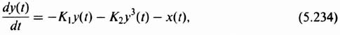
where K1, and K2 are not both zero. Depending on the values of K1 and K2, stability or instability can result. For example, if K1 > 0 and K2 > 0, and V(t) is given by
this system is stable, because the derivative of V(t) with respect to time t, dV(t)/dt, is negative, because

Equilibrium occurs at the singularity located at the origin, and the equilibrium point is asymptotically stable.
It is left as an exercise to the reader to prove that the condition K1 < 0 and K2 < 0 corresponds to an unstable equilibrium; the condition K1 > 0 and K2 < 0 corresponds to a stable equilibrium only if 0 < y2(t) < |K1/K2|.
It is important to recognize that the stability conditions obtained from a particular V(t) function are usually sufficient, but not necessary. In addition, a Liapunov function for any particular system is not unique. Therefore, if a particular V(t) function should fail to demonstrate whether a particular system is stable or not, there is no assurance that another function could not be found that does determine stability or instability. There is also no assurance that exceeding the limits based on a particular V(t) function will actually cause the equilibrium to be unstable. The Liapunov stability criterion is a conservative one.
As can be seen from this presentation, the primary use of Liapunov's second method is not the determination of stability where the answer may be found by other means, but is rather in the study of problems of stability which are not readily determined by other methods.
5.21. POPOV'S METHOD
An interesting and very powerful stability criterion for nonlinear control systems that are time invariant was introduced in 1959 by V. M. Popov, who obtained a frequency-domain criterion as a sufficient condition for asymptotic stability of single-loop control systems [13–20]. The method, as originally developed by Popov, is applicable to single-loop feedback systems containing time-invariant linear elements and time-invariant nonlinearities. An important feature of Popov's approach is that it is applicable to systems of high order. Once the frequency response of the linear element is known, very little additional calculation is required for determining stability of the nonlinear control system. It is an extension of the Nyquist diagram (see Section 1.7) to nonlinear systems.
This section presents Popov's stability criterion in terms of inequality constraints on the nonlinear element in conjunction with a modified frequency plot of the linear element. It will be shown that the most important and appealing feature of the Popov criterion is that it shares all of the desirable characteristics of the Nyquist method.
In order to introduce Popov's method, let us consider the nonlinear control system illustrated in Figure 5.71. It is composed of a linear, time-invariant process G(s) and a nonlinear, time-invariant element N[e(t)]. The reference input r(t) is assumed to be zero. Therefore, the response of this system can be expressed as
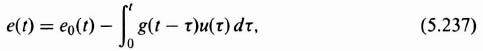
where

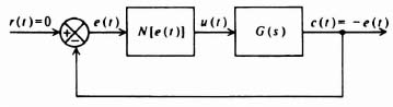
Figure 5.71 Nonlinear control system considered by Popov [14].
In this analysis, special restrictions are placed on the nonlinear and linear elements. For the nonlinear element n[e(t)], it is assumed that the input-output relationship is restricted to lie within the region illustrated in Figure 5.72 where
and
Furthermore, it is assumed that for all t, and for every finite value em there is a finite value um such that
The only assumption concerning the linear element G(s) is that it is output stable of degree n for some value of n. By this we mean that if n < 0, the output response to an initial condition or an impulse may diverge, but when the output is multiplied by ent it will converge towards zero. For the case of n > 0, output stable means that the output response to an initial condition or an impulse will converge towards zero faster than the function e−nt. In general, a linear element will be output stable of degree n if its transfer function G(s) and initial condition response function E0(s) are rational functions of s and its poles all satisfy
![]()
Therefore, n actually represents the settling rate of the linear element.
Popov's method is concerned with the asymptotic behavior of the control signal u(t) and output −e(t) of the linear element. Therefore, in addition to the definitions of asymptotic stability, local stability, finite stability, and global stability that were introduced in Section 5.20 in connection with the Liapunov stability criterion, we are concerned here with control asymptoticity and output asymptoticity. Control asymptoticity of degree n exists if a real value n can be found such that for every set of initial conditions
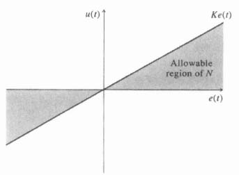
Figure 5.72 Restricted region of nonlinearity.

Output asymptoticity of degree n exists if a real value n can be found such that for every set of initial conditions
These stability definitions can be clarified by considering the following lemma.
If the linear element G(s) of Figure 5.71 is output stable of degree n, the input and output of the nonlinear element are bounded and satisfy Eq. (5.240), and the feedback system is control asymptotic of degree n, then
Therefore, if this lemma is satisfied, e(t) converges towards zero faster than e−nt for n > 0.
How can we relate control asymptotic and output asymptoticity? Obviously there should be some relationship based on the properties of the linear element G(s). Let us assume that the linear element is output stable of degree n. It can be shown that if the linear element is control asymptotic of degree n, then it is also output asymptotic of degree n. In addition, if for each set of initial conditions a number Q0 exists such that
![]()
then there exists a number Q that is dependent on Q0 such that
![]()
for all values of t. This appears reasonable because a decaying control signal u(t) that satisfies Eq. (5.241), when it is fed into the linear element whose unit-impulse response decays like u(t), will produce an output −e(t) that also decays in a similar manner.
Popov's fundamental theorem is based on the basic feedback control system illustrated in Figure 5.71. It is assumed that the linear system is output stable. The theorem states that for the feedback system to be absolutely control and output asymptotic for
![]()
it is sufficient that a real number q exists such that for all real ω ![]() 0 and an arbitrarily small δ > 0, the following condition is satisfied:
0 and an arbitrarily small δ > 0, the following condition is satisfied:
The relation (5.244) is the Popov criterion. Depending on the type of nonlinearity present, the following restrictions on q and K are imposed:
- For a single-valued time-invariant nonlinearity:

- For a nonlinearity having passive hysteresis (see Figure 5.73):
- For a nonlinearity having active hysteresis (see Figure 5.74):
Examination of these three possible types of nonlinearities shows that the theorem allows for a tradeoff between the requirements on the nonlinear and linear elements.
Let us rewrite Eq. (5.244) as follows:
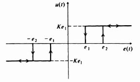
Figure 5.73 Passive hysteresis nonlinear characteristics.
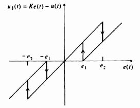
Figure 5.74 Active hysteresis nonlinear characteristics.
Relation (5.245) states that for each frequency ω, the Nyquist plot of G(jω) must lie to the right of a straight line given by
This line is called the Popov line and is illustrated in Figure 5.75. The angles α and β are
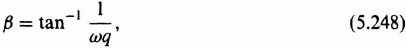
and it is clear that the slope of this line depends on the product ωq.
Stability depends on choosing a value of q such that, for each frequency ω, G(jω) lies to the right of the Popov line. It is important to recognize from Eqs. (5.247) and (5.248) that the slope of this line is frequency dependent. A Popov line whose slope is not frequency dependent can be found in a modified frequency plane. In order to find the particular frequency-insensitive Popov line, a simple transformation is used. The modified frequency response function G*(s) is defined as
Therefore, Eq. (5.245) can be rewritten as
In the G*(jω) plane, the Popov line is defined by
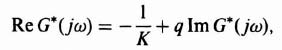

Figure 5.75 Popov's method when q is finite.
and is frequency insensitive. The Popov line in the G*(jω) plane is illustrated in Figures 5.76 and 5.77. The angle γ is defined as
![]()
Notice from Figures 5.76 and 5.77 that the G*(jω) locus passes to the right of a tangent to the locus at the point where G*(jω) intersects the negative real axis. These points are labeled −1/K. Therefore, K represents the maximum permissible gain for the system. For the case where q = 0, the Popov line expression reduces to
![]()
and the system is stable if it lies to the right of a vertical line passing through the point −1/K1 as is illustrated in Figure 5.76. Notice that the case of q = 0 gives the most conservative value of gain permissible.

Figure 5.76 Popov line in the G*(jω) plane for the case where q ![]() 0.
0.
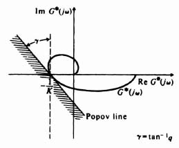
Figure 5.77 Popov line in the G*(jω) plane for the case where q < O.
A. Example 5.21-1
As an example of applying Popov's method, consider the system illustrated in Figure 5.78. For the linear element, the initial condition response e0(t) is given by
![]()
where e10, e20, and e30 depend on the initial conditions. The unit impulse response g(t) is given by
where U(t) is a unit step function. Equation (5.251) indicates that the linear element is output stable and satisfies one of the necessary constraints in order to use Popov's method. The corresponding G*(jω)-locus is illustrated in Figure 5.79. From this diagram, we can conclude that if the nonlinear element corresponds to a single-valued nonlinear element, and if q = 0.5, the Popov condition is satisfied when 0 < K ![]() 60.
60.
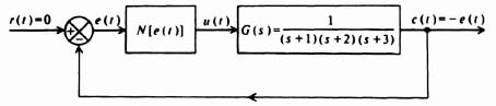
Figure 5.78 Nonlinear control-system example.
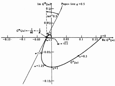
Figure 5.79 Popov analysis for system illustrated in Figure 5.78.
In conclusion, we see that the Popov method gives an exact and sufficient condition for determining the absolute stability of feedback systems having the configuration illustrated in Figure 5.71, with certain restrictions imposed. The inequality (5.244), which was given in terms of G(jω) which makes the technique easily applicable to systems having high-order processes which are to be controlled. In addition, the method shares all of the desirable characteristics of the Nyquist method. In the following section, Popov's method is extended to other types of systems which are not necessarily restricted to systems in which the linear portion is output stable, and the nonlinearity is time invariant.
5.22. GENERALIZED CIRCLE CRITERION
The generalized circle criterion [17, 18] enables ones to investigate the asymptotic behavior of a much wider class of systems than that for which Popov's theorem was originally intended. For example, this techique can be applied to systems having unstable or nonasymptotically stable plants, and time-variable nonlinearities. The generalized circle criterion presented in this section consists of modifying Popov's basic theorem in such a manner that the Popov condition can be applied directly to the original transfer function.*
Let us reconsider the basic nonlinear control system illustrated in Figure 5.71, and allow the nonlinearity to be time variable. It is assumed that the linear element of this system is not output stable. The generalized circle criterion is as follows: for the system of Figure 5.71 to be absolutely control and output asymptotic for
![]()
then it is sufficient that a real number q exist such that for all real ω, the following conditions are satisfied:

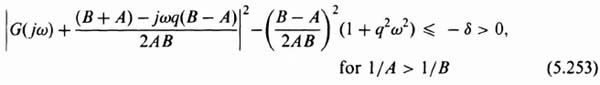
The quantitres B − A and q are restricted as K and q were in Popov's method, discussed previously in Section 5.21.
Figure 5.80 illustrates the physical interpretation of relation (5.252), where it is assumed that 1/A > 1/B. For each value of ω ![]() 0, the Nyquist plot of G(jω) must lie outside the circle centered at†
0, the Nyquist plot of G(jω) must lie outside the circle centered at†
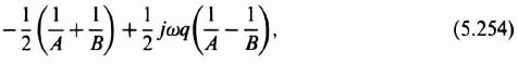
which crosses the real axis at the points −1/A and −1/B. It is interesting to note that if 1/B > 1/A, then the Nyquist plot must lie inside the circle that is centered at the point given by Eq. (5.254).
Analysis of the generalized circle criterion is quite interesting. For example, if we let A → 0 and B → K, then relations (5.252) and (5.253) reduce to (5.245) which corresponds to the Popov condition (5.244). On the other hand, if we let A → C and B → C, then we have a linear time-invariant system with gain C. For this case, the critical circle reduces to a point −(1/C) in the G(jω) plane, which is of course the critical point for the Nyquist diagram.
The generalized critical circle illustrated in Figure 5.80 and defined by Eqs. (5.252) and (5.253) is a function of frequency. Although all of the circles pass through the points −1/A and −1/B, their centers move up with increasing values of qω. However, for the general nonlinearity case where the nonlinearity may contain hysteresis and is time variable, q = 0 and a set of circles results that are symmetrical about the real axis. Notice also from Figure 5.80 that tradeoffs can be made between the requirements on the linear and nonlinear elements. For example, by narrowing the sector
the critical circles will be reduced and this will increase the permissible range of G(jω).
Let us consider the application of the generalized circle criterion. Unlike the situation for the Popov line of Section 5.21, it is not advantageous to transform the critical circles from the G(jω) plane into the G*(jω) plane, because this will only result in a family of curves that are not circles and whose shapes depend on both ω and q. However, it can easily be shown that if a tangent is drawn on the critical circle at the point −1/B, its angle α is given by

Figure 5.80 The generalized circle criterion for the case 1/A > 1/B.

Figure 5.80 illustrates this angle and also the angle which is given by
Comparing Figures 5.75 and 5.80, we observe that the tangent line on the critical circle has the same slope as the Popov line when A = 0. In addition, if
![]()
and
![]()
then the tangent line on the critical circle becomes identical to the Popov line shown in Figure 5.75. We also showed in Section 5.21 that the Popov line could be transformed into a frequency-independent line on the G*(jω) plane as was shown in Figures 5.76 and 5.77. Therefore, if G*(jω) lies to the right of the Popov line of Figures 5.76 and 5.77, then G(jω) lies outside the critical circle illustrated in Figure 5.80 for all ω.
A. Example 5.22-1
As an example of the generalized circle criterion, let us consider a nonlinear control system that is time variable in the configuration illustrated in Figure 5.71, where the transfer function of the linear element is given by
and the initial-condition response is
where e10, e20, and e30 are related to the initial conditions for a particular set of state variables. It is important to recognize that we are dealing with a nonlinear element that is time variable and a linear element that is not output stable, a problem which could not be solved using Popov's basic method. It is assumed that the nonlinear element corresponds to the general nonlinearity N[e(t), t], and therefore q must be chosen equal to zero. The solution consists of plotting the frequency locus G(jω) as is illustrated in Figure 5.81. The generalized circle criterion results in Popov sectors
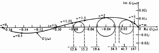
Figure 5.81 Generalized circle criterion example where
![]()
and the nonlinearity corresponds to the general time variable nonlinearity case where q = 0.
such that for each of these Popov sectors the G(jω) locus lies on or outside a circle symmetrical about the real axis and passing through the points −1/A and −1/B. For this particular example, the possible Popov sectors (illustrated in Figure 5.81) which result in stable systems are given by the following conditions:

Notice from Figure 5.81 that the size of the Popov sector, B – A, i.e., the difference between the lower bound A and upper bound B, depends on the size of the critical circle.
Therefore, we see that Popov's method can be extended to systems with unstable or nonasymptotically stable plants and time-varying nonlinearities by utilizing the generalized circle criterion. As shown in this section, the method permits the design of nonlinear systems whose linear elements are not output stable and whose nonlinearity can be time variable and correspond to any general nonlinearity. There are many practical situations where this is the very case involved, and the generalized circle criterion provides a very powerful method for solving this class of problems.
5.23. GUIDELINES FOR SELECTING THE “BEST” NONLINEAR CONTROL SYSTEM METHOD(S) PRESENTED FOR ANALYSIS AND DESIGN
Having learned the various methods available for analyzing nonlinear control systems in this chapter, how should the control-system engineer proceed for a specific problem? Which of the methods presented would you use? Unless guidelines are established for their use, uncertainty may exist as to the best approach(es) to be used in analyzing a nonlinear control system. This section provides guidelines for logically determining which analysis procedure(s) should be used in analyzing the stability of a particular nonlinear control system. These guidelines have been structured as a logic flow diagram, which is shown in Figure 5.82 [26]. This logic flow diagram should prove to be very valuable for integrating the various methods presented, and should prove useful to the student and the practicing control-system engineer.
In quasilinear systems, defined as those systems where the deviation from linearity is not too great, linear approximations may allow the use of conventional linear methods of analysis such as the Nyquist diagram, Bode diagram, or the root-locus method. This approach recognizes that certain control-system characteristics can change from one operating point to another, but it assumes that the control system is linear in the area of a specific operating point. For these control systems, the control-system engineer could use linear theory for analysis and design. This is the reason that linear theory has had such widespread use, although practical systems are never purely linear.
If the system cannot be approximated as a quasilinear system and linearizing approximations cannot be used, then we must use one or more of the nonlinear methods presented in this chapter for analysis and design.
If the linear and nonlinear portions of the system are time invariant, and the linear portion is stable (none of its roots are in the right half of the s-plane), then the describing function is recommended. Although it approximates a linearized transfer function by only considering the fundamental component of the output, it is a very powerful approach. Because of its approximation, it is essential that the method be checked by using an additional method. Simulation and the other nonlinear methods presented in this chapter can be used to check the describing function results.
If the nonlinear control system is second order, then the phase-plane and Liapunov methods are the most appropriate methods to use as a check. The Liapunov method could also be used as a check if the system were third order. If the system is third order or more, then Popov's method in the frequency domain can be used to determine asymptotic stability.
If the linear element is nonasymptotically stable, and the nonlinear element is time varying, then we can use the generalized circle criterion. This will determine allowable nonlinear gain ranges for system stability.
I always recommend that the nonlinear control system be simulated as a final check on system stability. It will assist in the check for factors which range from possible uncertainty regarding the validity of the assumptions, to analytic difficulties caused by system complexity. Simulation may also be necessary because of the failure of a technique to demonstrate stability conclusively. An example of this may be in the application of Liapunov's second method. The Liapunov condition for this method is sufficient, but not necessary, for stability. Therefore, failure to find a Liapunov function does not imply that the nonlinear control system is unstable. As noted in Figure 5.82, the simulation method is optional in some cases and, accordingly, it is shown as a dashed line for these cases.
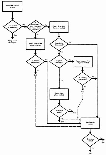
Figure 5.82 Logical approach for selecting method of analysis of nonlinear control systems [26]. (Reprinted from Control Engineering, October 1961, Copyright © 1961 Cahners Publishing Company).
5.24. ILLUSTRATIVE PROBLEMS AND SOLUTIONS
This section provides a set of illustrative problems and their solutions to supplement the material presented in Chapter 5.
- I5.1. A unity-feedback control system contains a linear element, G(s), and a nonlinear element containing a dead zone. The transfer function of the linear element is given by
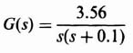
Assume that K1 in Figure 5.6 equals 1 for the dead zone. Using the describing-function method on a gain-phase diagram, determine the existence of any limit cycles.
SOLUTION: The gain-phase diagram for this nonlinear control system is illustrated in Figure I5.1. It was obtained using MATLAB. The −1/N curve was obtained from Figure 5.8. The gain-phase diagram shows that the system does not have a limit cycle, and it is stable. In addition, it can be concluded that the system is stable regardless of the size of the dead zone.
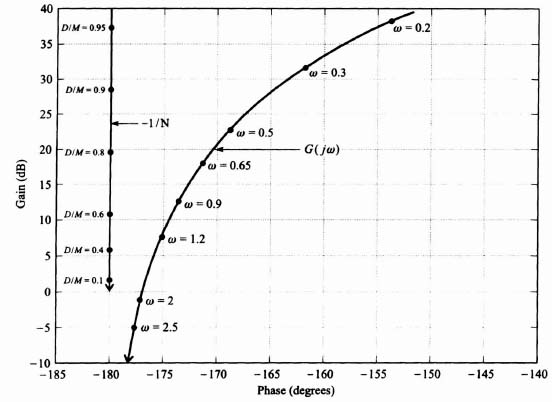
- I5.2. The following “bang-bang” control system represents the attitude-control system for an orbiting space satellite in which the reaction-jet moment u(t) is applied in a “bang-bang” manner. Determine the state equations of this nonlinear system.

SOLUTION:

Let
Therefore, the state equations are given by:

where the nonlinear relationship between u(t) and e(t) depends on the sign of e(t) = r(t) − c(t) as follows:
Therefore, the state equations are given by:
- I5.3. The phase trajectory for the previous problem analyzed in Illustrative Problem I5.2 is to be determined.
- Determine the phase trajectory equation for this “bang-bang” control system by using the method of transforming the second-order differential equation to a first-order differential equation. Assume that x1(0) and x2(0) are the initial values of the states and the reference input is a constant equal to r0.
- Draw the phase trajectory of this control system and determine what occurs when x1(t) < r0 and what occurs when x1(t) > r0.
SOLUTION:
- Dividing Eq. (I5.2-2) by (I5.2-1) from Illustrative Problem I5.2, we obtain the following:
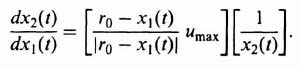
Separating the two variables, x1(t) and x2(t), and integrating we obtain the following:
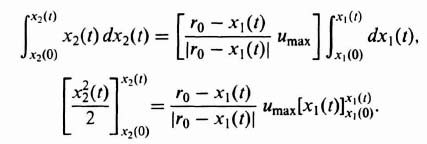
Therefore, the trajectory equation is given by:

- When x1(t) < r0, then

When x1(t) > r0, then
Therefore, these two resulting trajectories represent two sets of parabolas. For the arbitrary initial conditions given, x1(0) and x2(0), the trajectories are sketched as follows and we observe that a limit cycle occurs:
There is one additional important point to make in this illustrative problem. For the initial condition given at state x(0), we note that x1(0) is less than r0. The question arises as to whether the trajectory leaves the initial state, x1(0), and moves to the right or left. This question can be answered by reconsidering the state equation of this system given in Illustrative Problem I5.2 by Eq. (I5.2-1):
Because both x2(0) and dt are positive, then dx1(t) must also be positive and the motion along the trajectory must be to the right.
At x(t1), x1(t) now equals r0 and as x1(t) becomes greater than r0, the relay switches and we transfer to the new trajectory. The motion along this new trajectory continues until we reach state x(t2) and we again switch back to the original trajectory. The system then returns to its original state at x(0). This periodic oscillation, or limit cycle, will continue unless the reference input r0 changes.
- I5.4. The phase plane for the nonlinear control system shown in Figure I5.4 containing a nonlinear element containing a dead zone and saturation is to be determined using the method of isoclines.
- Determine the general expression for the isocline equations. Assume the reference input, r(t) is a constant r0.
- Plot the phase trajectory for e(0) = 2 using the isocline method.
SOLUTION:
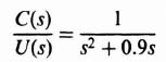
Therefore,
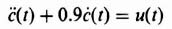
where

where

Therefore,
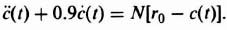
Because N(e(t)) is a function of e(t) rather than c(t), we will define the states in terms of e(t) and
 rather than c(t) and
  . Therefore, let the states be defined as:
Therefore, the state equations are given by:
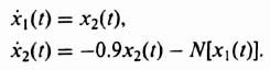
Therefore, the isocline equations are given by:
- Region 1: If e(t) = x1(t) > + 1, then N[e(t)] = N[x1(t)] = 1. In this case the isocline equation, Eq. (I5.4-1) is given by
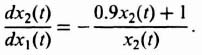
Because the isocline equation is independent of x1(t), the isoclines are all horizontal lines.
Region 2: If −1 < e(t) < 1, then N[e(t)] = N[x1(t)] = 0. In this case the isocline equation, Eq. (I5.4-1), is given by

In Region 2, all trajectories have a slope of −0.9.
Region 3: If e(t) = x1(t) < −1, then N[e(t)] = N[x1(t)] = −1. In this case the isocline equation, Eq. (I5.4-1), is given by
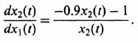
As in Region 1, since the isoclines are independent of x1(t), the isoclines are all horizontal lines [see Figure I5.4(ii)].

- I5.5. In the following nonlinear control system, the control input, u(t), is proportional to the error and it contains a nonlinear component f(e) depending on the derivative of the error as follows:
- Determine the state equations of this nonlinear control system. Assume that the reference input, r(t), is constant. Define the state variables x1(t) and x2(t) in terms of e(t) and de(t)/dt, respectively, in this problem.
- Determine whether the system is stable using Liapunov's second method.
SOLUTION:
- For the linear portion of this control system,

Substituting the value of u(t) given in the problem, we obtain the following:
Since e(t) = r(t) − e(t) and since r(t) is a constant, we can rewrite this equation as:
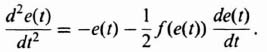
Defining the states as x1(t) = e(t) and x2(t) = de(t)/dt, the state equations are given by:
- Let the energy function V(t) be given by
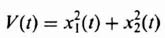
Therefore,
Substituting the state equations (I5.5-1) and (I5.5-2) into the derivative of the energy function, Eq. (I5.5-3), we obtain the following:
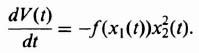
Because

is always positive, then
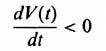
and the system is asymptotically stable if

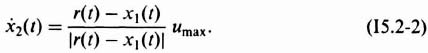

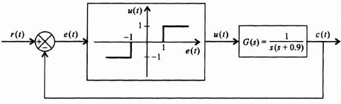
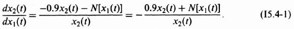
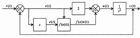
PROBLEMS
- 5.1. The torque speed characteristics of a two-phase, ac instrument servomotor are illustrated in Figure P5.1. Assume that the inertia of the rotor is 0.1 oz in2 and that the load inertia and coefficient of viscous friction are negligible.

- Derive the transfer function of the motor, relating output position to control voltage using linearizing approximations. Approximate the characteristics by one straight line that is tangent to the exact characteristics at 1000 rpm, and by one straight line that goes through the two endpoints. Compare your results.
- How do the time constants derived in (a) change if the torque speed characteristics are approximated by two other straight lines: one at low speed that is tangent to the exact characteristics at 250 rpm, and one at high speed that is tangent to the exact characteristics at 1750 rpm.
- Comparing your answers to (a) and (b), what conclusions can you reach?
- 5.2. Derive the describing function corresponding to the combined nonlinear characteristics of saturation S and dead zone D.
- 5.3. Derive the describing of a two-position contactor which does not exhibit any hysteresis effect.
- 5.4. An amplifying device in a feedback loop has the following nonlinear characteristics:
- No output signal for all inputs whose magnitude is less than E1 V.

- Input signals whose magnitude is greater than E1 V but less than E2 V are amplified according to the relation
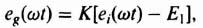
where
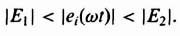
- For all input signals whose magnitude is greater than E2 V, the output is given by
when
Sketch the input–output characteristics and derive the describing function.
- No output signal for all inputs whose magnitude is less than E1 V.
- 5.5. Derive the describing function for an amplifying device which has the nonlinear characteristics illustrated in Figure P5.5.
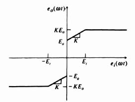
- 5.6. The characteristics of Figure P5.6 represent those of an on-off element (relay) having a dead zone D present. Determine the describing function for these relay characteristics assuming that the input to the nonlinear element is a sinusoid of m(ωt) = M sin ωt, Reduce your final answer so that it is only in terms of the nonlinear relay characteristics D and K1 and M.
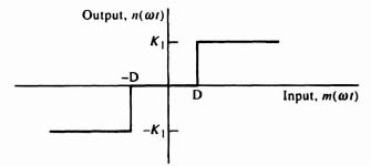
- 5.7. Determine the describing function for the nonlinear characteristic shown in Figure P5.7 consisting of a nonlinear dead zone and a linear gain, where the dead zone is represented by D and the gain is represented by K.

- 5.8. Determine the describing function for the nonlinear characteristic shown in Figure P5.8 consisting of a nonlinear Coulomb friction and linear viscous friction. The Coulomb friction level, which opposes velocity, is represented by Fc, and the linear vicous friction is represented by B. The input to this nonlinear characteristic is velocity, and the output is represented by friction (torque).
- 5.9. An instrument servo system used for positioning a load may be adequately represented by the block diagram shown in Figure P5.9, which indicates that the system contains backlash.
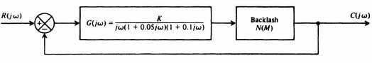
- Using the gain-phase diagram, determine the existence of any limit cycles if K = 25.
- What is the maximum gain that can be tolerated in G(jω) before a limit cycle occurs?
- 5.10. In contrast to the on-off element having dead-zone and hysteresis characteristics present, as analyzed in Figure 5.17, an ideal relay has no dead-zone or hysteresis characteristics.
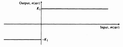
- For the ideal relay characteristics shown in Figure P5.10, determine its describing function analytically, assuming that the input to the nonlinear element is a sinusoid of M sin ωt.
- Check your answer by reducing Eq. (5.62) for the conditions of zero dead zone and hysteresis [A1 of Eq. (5.61) now becomes zero]. Do your answers agree?
- 5.11. Utilizing the result of your derivation of the describing function for the ideal relay characteristics in Problem 5.10, consider the stability of the control system shown in Figure P5.11. For the value of G(jω) indicated, determine the existence of any limit cycles and whether they are stable or unstable. Assume K1 = 1.
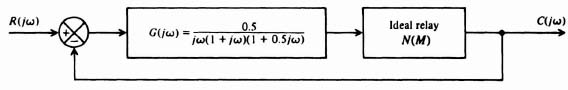
- 5.12. Repeat Problem 5.11 for
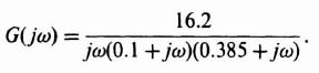
Assume k1 = 1.
- 5.13. Assume that the block diagram of a load-positioning control system, which contains backlash, is represented as in Figure P5.9 and that the linear portion's transfer function is given by
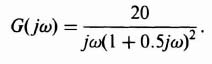
- Using the gain-phase diagram, determine the existence of any limit cycles. Are the limit cycles stable or unstable?
- Determine the gain which can perrnit a stability margin of 6 dB.
- 5.14. Repeat Problem 5.13 for
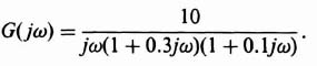
Use a stability margin of 3 dB in part (b).
- 5.15. Repeat Problem 5.13 for

- 5.16. A unity-feedback control system contains a nonlinear element containing backlash, N(M), and a linear device whose transfer function is given by
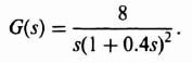
- Using the gain-phase diagram, determine the existence of any limit cycles. If any limit cycles exist, determine the frequency ω and D/M at the intersection(s).
- Determine the gain which can permit a stability margin of 6 dB.
- It is desired to stabilize this control system by the introduction of rate feedback as shown in Figure 5.30. Determine the rate-feedback constant b which will permit a stability margin of 6°.
- 5.17. A unity-feedback system consists of cascaded elements which include a relay, pure integration, an amplifier which saturates, a two-phase ac servomotor, and a gear train containing backlash.
- Draw the block diagram and show the linear transfer functions and the describing functions for the nonlinear elements, symbolically.
- Qualitatively illustrate how you would predict the presence of an oscillation on a gain-phase diagram.
- 5.18. A unity-feedback instrument servo with a spring-loaded shaft has a dead zone of 2°. Assume that K1 in Figure 5.6 equals 1. The transfer function for the linear portion of the system is given by
Utilizing the describing-function method on a gain-phase diagram, determine the conditions necessary for the existence of a limit cycle.
- 5.19. An instrument servo contains a three-position contactor which has a pull-in point and a drop-out point at errors of 0.02 and 0.01 rad, respectively. The transfer function of the linear portion of the unity-feedback control system is given by

Determine whether a limit cycle exists using the describing-function analysis on a gain-phase diagram. Assume that K1 in Figure 5.17 equals 1.
- 5.20. Repeat Problem 5.18 with the transfer function for the linear portion of the system given by
- 5.21. A unity-feedback instrument servo is driven by an amplifier which saturates at 70% of rated voltage of the motor. Assume that the gain of the unsaturated amplifier is 40. The transfer function of the linear portion of the system, excluding the amplifier, is given by
Utilizing the describing-function method on a gain-phase diagram, determine whether a limit cycle exists.
- 5.22. An instrument servo contains a three-position contactor which has a pull-in point and a drop-out point at errors of 0.03 and 0.01 rad, respectively. The transfer function of the linear portion is given by
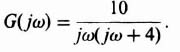
Determine whether a limit cycle exists utilizing the describing-function analysis on a gain-phase diagram. Assume K1 in Figure 5.17 equals 1.
- 5.23. Repeat Problem 5.22 with the transfer function of the linear portion given by
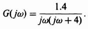
- 5.24. The rate-control system shown in Figure P5.24, using a tachometer for feedback, has a nonlinear element containing a dead zone of 2°. Assume that K1 in Figure 5.6 equals 1. The transfer function of the linear element can be approximated as
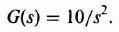
Using the describing-function method on a gain-phase diagram, determine whether any limit cycles occur.
- 5.25. The Orbiting Astronomical Observatory (DAD), shown in Figure P5.25a, is designed to provide astronomers with a standardized stable platform in space readily adaptable to a variety of experiments [42]. Orbiting at 500 miles altitude, the DAD permitted scientists to examine any point in the heavens, unimpeded by the Earth's atmosphere. In addition, it has a precision and stability unsurpassed even by a stationary observatory. After injection into orbit and separation of the satellite from the second booster stage, the high-thrust gas jets stop any tumbling or rolling sensed by rate gyros and align the

Figure P5.25 (a) NASA's OAO being checked out at Cape Kennedy. (Official NASA photo) (b) Equivalent block diagram of the roll coarse solar orientation control loop.
OAO's optical axis with the Earth-Sun line to
 . The OAO utilizes coarse and fine solar orientation control systems. The coarse loop depends on gas jets firing and is a nonlinear control system. The fine loop depends on a momentum-exchange wheel and is a linear control system. Let us consider the nonlinear characteristics of the coarse solar orientation control system in this problem. Figure P5.25b illustrates an equivalent block diagram of the roll coarse solar orientation control loop. Basically, it consists of a switching amplifier which has very similar characteristics to the nonlinear on-off element having hysteresis that has been analyzed previously and which controls a solenoid valve and jet. As indicated in Figure P5.25b, the jet fires when the error reaches ±3 V and stops firing when the error is reduced to ±2.9 V. Assume that the resultant corrective torque produced by the jet is ±0.3 lb ft, and the inertia in the roll axis is 1000 lb ft sec2. The rate gyro which closes this rate loop, has a sensitivity of 10V/(degree/sec). Using the describing-function analysis on a gain-phase diagram, determine the existence of any limit cycles.
 - 5.26. An instrument servo system used for positioning a load may be adequately represented by the block diagram shown in Figure P5.26.
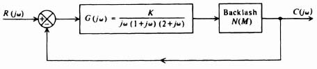
- Using the gain-phase diagram, prove that if K = 4 the system exhibits a limit cycle(s). Determine the range of frequencies and D/M ratios for which the limit cycle(s) exist. Are they stable or unstable?
- It is desired to stabilize this configuration by reducing the system gain. Determine the maximum value of gain K which will allow a minimum stability margin of 2 dB.
- It is desired to stabilize this configuration by adding a phase-lead network in cascade with G(jω). Determine the time constants of the lead network

which will permit a minimum stability of 5°.
- It is desired to stabilize this configuration by the introduction of rate feedback as shown in Figure 5.30. Determine the rate-feedback constant b which will permit a minimum stability margin of 6°.
- 5.27. Repeat Problem 10.26 for

- 5.28. Repeat Problem 10.26 for
For part (d) to this problem, design for a minimum stability margin of 5°.
- 5.29. The control system shown in Figure P5.29 uses an ideal relay to apply a corrective signal of the proper phase to control the position of a servomotor. This type of nonlinear control system, which does not use an amplifier, is popularly known as a “bang-bang” control system.

Using the result of your derivation of the describing function for the ideal characteristics in Problem 5.10 [or by reducing Eq. (5.62) of the textbook for the condition of zero dead zone and hysteresis), consider the stability of the control system shown. Determine the existence of any limit cycles, and whether they are stable or unstable. Assume K1 = 1.
- 5.30. A positioning system consists of a major feedback path and three minor feedback paths as shown in Figure P5.30. Utilizing the signal-flow graph and describing-function approaches, determine whether any limit cycles exist if the nonlinearity corresponds to backlash and the system parameters correspond to the following values:

- 5.31. Repeat Problem 5.30 with the nonlinearity corresponding to Coulomb friction.
- 5.32. In 1965 the Ranger unmanned space vehicle, shown in Figure P5.32a investigated the surface of the moon by means of a TV camera and instruments.
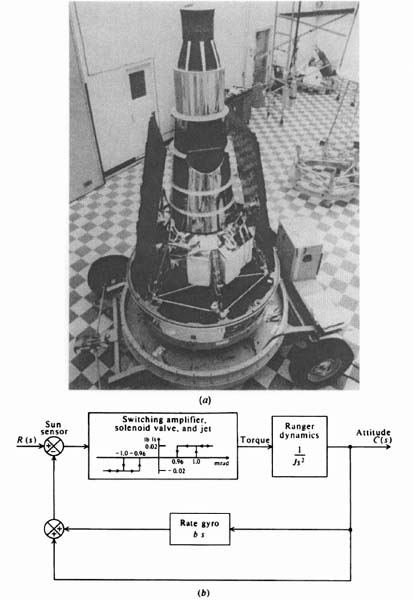
Figure P5.32 (a) Ranger spacecraft being checked out at Cape Kennedy. (Official NASA photo) (b) Equivalent block diagram of the Ranger attitude control system for the pitch axis.
From a control-system viewpoint, the Ranger attitude-control system must stabilize the vehicle from second-stage separation until lunar encounter [43]. The accuracy requirements are especially high, because the Ranger vehicle is an unmanned vehicle and its solar panels must point accurately at the Sun in order to obtain energy. In addition, the Ranger vehicle transmits data back to Earth by means of a narrow-beam antenna which requires very accurate pointing. The equivalent block diagram of the Ranger attitude-control system for the pitch axis is illustrated in Figure P5.32b. Error signals in position, generated by a sensor, are added to velocity error signals generated by a rate gyro. A switching amplifier, which has very similar characteristics to the nonlinear on-off element having hysteresis that has been analyzed previously, controls a solenoid valve and jet. As indicated in Figure P5.32b, the jet fires when the dead-zone error is equivalent to ±1 mrad and stops firing when the error decreases to ±0.96 mrad. Assume that the corrective torque produced by the jet is ±0.02 lb ft, and the inertia of Ranger in the pitch axis is 110 lb ft sec2. Utilizing the describing-function method, determine the existence of any limit cycles.
- 5.33. The block diagram of a load positioning control system containing backlash is shown in Figure P5.33a.

- Using the describing-function analysis (on a gain-phase diagram), determine the existence of any limit cycles.
- It is desired to stabilize this configuration by the introduction of rate feedback as shown in Figure P5.33b. Design the rate-feedback constant b for a minimum margin of stability of 20°.
- 5.34. Repeat Problem 5.33 for

In part b of this Problem, design the rate feedback constant b for a minimum margin of stability of 12°.
- 5.35. The control system of Figure P5.35 illustrates an undamped servo, where the motor torque is proportional to the error e(t) and is not affected by velocity. Consider the composite gain of the forward part of the loop to be 800 dyne cm per radian of error.
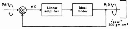
- Draw the phase trajectory for the following set of initial conditions:

- What conclusions can you reach from the phase trajectory?
- Draw the phase trajectory for the following set of initial conditions:
- 5.36. The control system shown in Figure P5.36 illustrates a positioning servo system.

- Draw the phase trajectory for the following set of initial conditions:
- What conclusions can you reach from the phase portrait?
- Draw the phase trajectory for the following set of initial conditions:
- 5.37. Draw the phase portrait of a linear unity-feedback unexcited control system whose transfer function is given by

- 5.38. Repeat Problem 5.36 with a rate limiter at −2 rad/sec added to the system.
- 5.39. Repeat Problem 5.36 with a position limiter at −0.5 rad added to the system.
- 5.40. Repeat Problem 5.37 with the rate limiters at ±1 rad/sec added to the system.
- 5.41. Repeat Problem 5.37 with position limiters at ±1 rad added to the system.
- 5.42. Determine the time it takes for the phase trajectory illustrated in Figure P5.42 to transverse the following segments: AB, BC, CD, DE, AE.
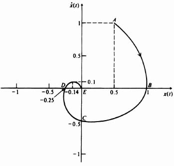
- 5.43. Manipulate the following equations into the form d
 /dθ = f(θ, t):
- 5.44. Derive the isocline equation for each of the following differential equations and draw the isoclines together with their slope markers:
- 5.45. Construct the phase portraits for each of the differential equations of Problem 5.44 using the method of isoclines.
- 5.46. Determine and construct the phase trajectory for a second-order system containing rate limiting where θ(0) = 0.7 and
 = 0. The differential equation for the system is given by
and

- 5.47. Repeat Problem 5.46 for the same second-order differential equation, but with the initial conditions given by θ(0) = 1 and
 = 0 and rate limiting given by
- 5.48. A linear unity-feedback control system contains a forward transfer function given by
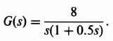
- Draw the phase trajectory for the following set of initial conditions using the method of isoclines:
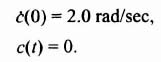
- What kind of singular point does the origin of the phase plane represent? What conclusions can you reach from this phase trajectory?
- A position limiter is added to the output of this control system at ±1.5 rad. How does this change the phase trajectory?
- Draw the phase trajectory for the following set of initial conditions using the method of isoclines:
- 5.49. Determine and construct the phase trajectory of a nonlinear control system for which the describing equations are given by
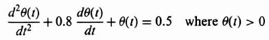
and
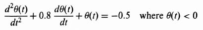
Assume that the initial conditions are θ(0) = 0.5 and (dθ(0)/dt) = 0.
- 5.50. A phase trajectory of a nonlinear control system is illustrated in Figure P5.50.

- Determine the time it takes to traverse the segment OA by direct integration.
- Determine the time it takes to traverse the segment DE by direct integration.
- 5.51. Using Liapunov's second method, determine the stability of the nonlinear control system described by the differential equation

- K1 > 0, K2 > 0
- K1 < 0, K2 < 0
- K1 < 0, K2 > 0.
- 5.52. Using Liapunov's second method, determine the stability of the nonlinear second-order control system described by the differential equation
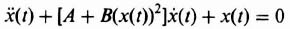
if
- A > 0, B > 0
- A < 0, B < 0
- A > 0, B < 0.
- 5.53. Repeat Problem 5.52 for

- 5.54. Using Liapunov's second method, determine the stability of the control system described by the nonlinear differential equation
Assume that K1 and K2 are positive constants.
- 5.55. Utilizing Liapunov's second method, determine the stability of the control system described by the nonlinear differential equation

if
- K1 > 0, K2 > 0
- K1 < 0, K2 < 0
- K1 > 0, K2 < 0
- 5.56. Repeat Problem 5.55 for the nonlinear differential equation

- 5.57. A unity-feedback control system contains a linear and nonlinear element. The transfer function of the linear element is given by

The initial-condition response of the linear element is given by
where e10, e20, e30, and e40 are related to the initial conditions and the unit-impulse response is given by

where U(t) is the unit step input. Using Popov's method, determine the values of K which will result in a stable system, assuming that the nonlinear element is single valued with q = 1.0.
- 5.58. Repeat Problem 5.57 with q = 0.75 and the transfer function of the linear element given by
- 5.59. The control system shown in Figure P5.59 contains a nonlinear element N[e(t)] and a linear element whose transfer function is G(s). Assume that the nonlinearity corresponds to a general, single-valued, nonlinear element, with q = 0, and whose gain can vary between 0 and a maximum value of K. Using Popov's method, determine the values of K which will result in a stable control system.
- 5.60. A unity-feedback control system containing a linear and nonlinear element is to be analyzed using Popov's method. The transfer function of the linear element is given by
The nonlinear element corresponds to the general nonlinearity case (q = 0)
- Determine the frequency ω where the imaginary part of G*(jω) is zero.
- Using Popov's method, determine the values of K which will result in a stable system.
- 5.61 Repeat Problem 5.57 with q = 1.11 and the transfer function of the linear element given by

- 5.62. A unity-feedback control system contains a linear and nonlinear element. The transfer function of the linear element is given by

The initial condition response is

where e10, e20, and e30 arise from the initial conditions. Using the generalized circle criterion, determine possible values of N[e(t), t] which will result in a stable system if the nonlinear element corresponds to the general nonlinearity case (q = 0).
- 5.63. Repeat Problem 5.62 with the transfer function of the linear element given by
- 5.64. Repeat Problem 5.62 with the transfer function of the linear element given by

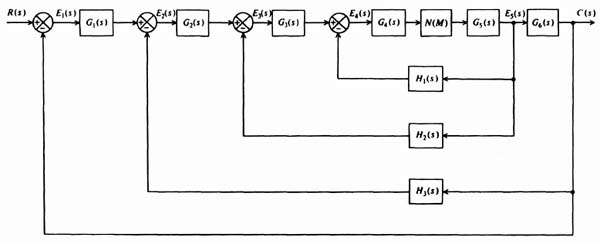

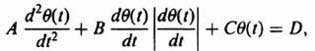


REFERENCES
1. P. M. Lowitt and S. M. Shinners, “Type N—Integral space tracking configuration.” IEEE Trans. Mil. Electron., MIL-9, 88–98 (1965).
2. A. M. Liapunov, On the general problem of stability of motion. Ph.D. thesis. Kharkov 1892; reprinted (in French) in Annals of Mathematics Studies. Vol. 17. Princeton University Press. Princeton, NJ. 1949.
3. N. Minorsky, Theory of Nonlinear Control Systems. McGraw-Hill, New York, 1969.
4. E. Levinson, “Some saturation phenomena in servomechanisms.” Trans. Am. Inst. Electr. Eng. 72, 1 (1953).
5. C. A Ludeke. “The generation and extinction of subharmonics.” In Proceedings of the Symposium on Nonlinear Circuit Analysis. Polytechnic Institute of Brooklyn, New York, 1953.
6. O. I. Elgerd, Control Systems Theory. McGraw-Hill, New York, 1967.
7. R. J. Kochenburger, “A frequency response method for analyzing and synthesizing contactor servo-mechanisms.” Trans. Am. Inst. Electr. Eng 69, 270 (1950).
8. E. C. Johnson, “Sinusoidal analysis of feedback-control systems containing nonlinear elements.” Trans. Am. Inst. Electr. Eng. 71, 169 (1952).
9. H. D. Grief, “Describing function method of servomechanism analysis applied to most commonly encountered nonlinearities.” Trans. Am. Inst. Electr. Eng. 72, 253 (1953).
10. J. G. Truxal, Automatic Feedback Control System Synthesis. McGraw-Hill, New York, 1955.
11. J. T. Leigh, Essential of Nonlinear Control Theory. Peter Peregrinus Ltd., London, 1983.
12. E. Levinson, “Phase-plane analysis.” Electro-Technology 69, 118 (1962).
13. C. A Desoer, “A generalization of the Popov criterion.” IEEE Trans. Autom. Control AC-10, 182–185 (1965).
14. V. M. Popov, “Absolute stability of nonlinear systems of automatic control.” Autom. Remote Control (USSR), 22, 857–875 (1961).
15. V. A Jakubovic, “Frequency conditions for the absolute stability and dissipativity of control systems with a single differentiable nonlinearity.” Sov. Math. Engl. Transl. 6, 98–101 (1965).
16. S. Lefschetz, Stability of Nonlinear Control Systems. Academic Press, New York, 1965.
17. J. C. Hsu and A. U. Meyer, Modern Control Principles and Applications. McGraw-Hill, New York, 1968.
18. G. Zames, “On the input-output stability of time-varying nonlinear feedback systems. Part II. Condition involving circles in the frequency plane and sector nonlinearities.” IEEE Trans. Autom. Control, AC-11, 46–76 (1966).
19. V. M. Popov and A. Halanay, “On the stability of nonlinear automatic control systems with lagging argument.” Autom. Remote Control (USSR), 23, 783–786 (1963).
20. A. V. Michailov, “Harmonic analysis in the theory of automatic control.” A. T. Moscow, No. 3, p. 27, 1938.
21. B. O. Watkins, Introduction to Control Systems. Macmillan, New York, 1969.
22. H. H. Rosenbrick and C. Storey, Computational Techniques for Chemical Engineers. Pergamon, Oxford, 1966.
23. D. D. McCracken and W. S. Dorn, Numerical Methods and FORTRAN Programming. Wiley, New York, 1964.
24. R. W. Hamming, Numerical Methods for Scientists and Engineers. McGraw-Hill, New York, 1962.
25. S. M. Shinners, “Which computer—Analog, digital or hybrid?” Mach. Des., 43, 104–111 (1971).
26. S. M. Shinners, “Guidelines for the analysis of nonlinear control systems.” Control Eng. 28(11), 181–182 (1981).
27. D. P. Atherton, Nonlinear Control Engineering. Van Nostrand-Reinhold, London, 1982.
28. P. M. Lowitt and S. M. Shinners, “Integrated optimal synthesis for a radar tracker.” In Proceedings of the Seventh National Military Electronics Convention, Washington, DC, 74–78, September 1963.
29. MATLAB™ for MS-DOS Personal Computers User's Guide, Control System Toolbox MathWorks, Inc., Natick, MA, 1997.
30. A. Grace, A. J. Laub, J. N. Little, and C. Thompson, Control System Toolbox for Use with MATLAB™ User's Guide. MathWorks, Inc., Natick, MA, 1990.
31. J. M. Boyle, M. P. Ford, and J. M. Maciejewski, “Multivariable toolbox for use with MATLAB.” IEEE Control Syst. Mag. 9(1), 59–65 (1989).
32. D. Graham and D. McRuer, Analysis of Nonlinear Control Systems. Wiley, New York, 1961.
33. R. Oldenburger and R. C. Boyer, “Effects of extra sinuosoida1 inputs to nonlinear systems.” In Proceedings of the ASME Winter Annual Meeting, New York, 1961.
34. S. M. Shinners, “Dual-input describing function.” Control Eng. 18, 53–55 (1971).
35. O. I. Elgerd, “Continuous control by high frequency signal injection.” Instrum. Control Syst. 37, 12 (1964).
36. R. C. Boyer, Sinosoidal signal stabilization. M. S. Thesis, Purdue University, Lafayette, IN, 1960.
37. J. E. Gibson, Nonlinear Automatic Control. McGraw-Hill, New York, 1963.
38. J. A. Aseltine, W. R. Beam, J. D. Palmer, and A. P. Sage, Introduction to Computer Systems. Analysis. Design and Applications. Wiley, New York, 1989.
39. N. Stern and R. A. Stern, Introducing Quick BASIC 4.0 and 4.5: A Structured Approach. Wiley, New York, 1986.
40. S. A Hovanessian and L. A. Pipes, Digital Computer Methods in Engineering. McGraw-Hill, New York, 1969.
41. C. Belove, ed., Handbook of Modern Electronics and Electrical Engineering. Wiley, New York, 1986.
42. O. Romaine, “OAO: NASA's biggest satellite yet.” Space/Aeronaut. 40, 54–58 (1962).
43. W. Turk, Ranger Block III altitude control system. Jet Propul. Lab. Tech. Rep. No. 32–663, 1964.
*Asymptotic stability and nonlinear system stability classified in terms of a regional basis are discussed in Section 5.20, where Liapunov's stability criterion is presented.
†As far as control-system design is concerned, a steady oscillation is treated as being unstable,
*Nate that when linearizing along a trajectory, the matrics A and B will be functions of time.
*The dual-input describing function is a modified describing function which is dependent on two frequency components: the intelligence signal and the dither signal.
*A system described by an nth-order differential equation requires an n-dimensional phase space with a knowledge of n initial conditions. It is, indeed, ar arduous task to visualize this for third- and higher-order systems, and is rarely used.
*There are about 30 different classes of stability currently in use. However, the types defined in this book are the important ones most frequently used by the control-system engineer.
†The circle criterion was originally developed only for the case of q = 0 [18]. However, the generalized circle criterion presented here is an extension which is valid for all values of q including zero [17].