
This chapter is about working with surfaces in Civil 3D. Most land development and civil engineering projects wind up as surfaces eventually. This surface can be a water surface, the top of a new landfill, a rock layer, or airspace above an airport. Surfaces help engineers understand the relationships between the horizontal control data and the vertical elevation data.
In Civil 3D, you have a myriad of ways to interact with surfaces. In this chapter, you'll explore using surfaces as preliminary design tools and performing some basic land analysis. You'll then look at building surfaces from Google Earth, survey, and point information. You'll take this information and edit it for accuracy and clarity, including some labeling concepts. Then you'll look at how to use the analysis tools for preliminary engineering and earthworks.
This chapter includes the following topics:
Building surfaces from Google Earth
Building surfaces from point and contour data
Editing boundaries, breaklines, and bad data
Labeling surfaces for clear understanding
Analyzing surfaces for flood analysis and earthworks
When you're building a surface in Civil 3D or any other program, it's important to understand the limitations of most surface-based designs. When a program uses a surface, it's not the same as using a solid object. A surface is the skin of the object. Imagine if you could peel the color of an orange peel. You could look at and understand by the shape and color that it represents the orange, but you couldn't unwrap it and eat it. A solid has mass and thickness; a surface has neither. In addition, surfaces in Civil 3D recognize only a single elevation for any point in the coordinate system. This means you cannot model caves or overhangs with a single surface. Now that you're aware of the limits, let's look at all you can do with the surface object in Civil 3D.
At its core, Civil 3D builds surfaces from triangles. The exact methodology is based on the Delaunay algorithms, but Civil 3D then attempts to refine that triangulation based on user input and constraints. There are a number of essential building blocks that can be used to build and modify a surface:
Boundaries
Breaklines
Contours
DEM files
Points
In addition to these building blocks, you can also edit surfaces after they've been built by modifying the surface points, removing or rearranging triangles, thinning data, or moving the surface datum. We'll explore the most common methods in this chapter, but not all of them.
In this chapter, you'll look specifically at building surfaces from three main sources: Google Earth, surveyed point data, and drawing contour information. Each of them is valuable and has its place in the land-development process.
When Google Earth showed up on the scene, a lot of people reacted with, "Cool, but what do we do with it?" The original link between Civil 3D and Google Earth was nice for the demo shows, but there wasn't much meat to it. With the ability to create a surface directly from Google Earth data in Civil 3D, there's a real tool with a real purpose that can be used for real work.
Before you can import data from Google Earth (or any real-world coordinate system for that matter), you have to assign a coordinate system to your drawing. You'll walk through this process in the following short exercise.
Open the
Importing GE Surface.dwgfile (which can be downloaded fromwww.sybex.com/go/introducingcivil3d2010).Right-click the drawing name and select Edit Drawing Settings to open the Drawing Settings dialog.
If necessary, change to the Units and Zone tab.
In the Zone area, make the following changes:
Change the Zone to USA, Texas.
Change the Coordinate System to NAD83 Texas State Planes, South Central Zone, US Foot.
Your settings should now look like Figure 7.1
Click OK to close the dialog.
This sets the zone and coordinates for your new file. (For more information on these drawing settings, see Chapter 1, "Welcome to the Civil 3D Environment.") Now you need to find your site in Google Earth.
Launch Google Earth on your computer (but leave Civil 3D open in the background).
Once Google Earth has loaded, open the
Introducing Civil 3D.kmzfile by selecting File → Open and browsing to the Introducing Civil 3D dataset. A.kmzfile is basically a reference file telling Google Earth where to go in the world.Switch back to Civil 3D once the file is open.
Change to the Insert tab on the ribbon, and then on the Import Panel, select Google Earth → Import Google Earth Surface.
Press Enter to accept the command line option to use the coordinate system already in place in the drawing. This opens the Create Surface dialog.
Click OK to close the dialog, accepting the defaults and completing the exercise.
Switch back to Google Earth and exit that program.
Your screen should look like Figure 7.2. Note that the contours seem a bit rough in places. Look particularly at the northwest corner, where the staggered and rough contours would seem to indicate some surface refinement would be in order. These sorts of surface anomalies are quite common when using Google Earth data.
Close the drawing.

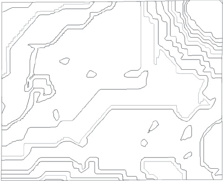
Although this data is accurate enough for most preliminary engineering or large-scale hydrology work, it should not be used for construction or bidding purposes. During informal testing, Google Earth data has been found to be as much as 15′ different from on-the-ground survey points in spots, while being dead-on in others. If you think of Google Earth data as similar to the topography maps provided by many governments, you'll have the right frame of mind toward its application.
Once you've moved beyond preliminary steps, it's time to get a bit more accurate and look at some other surface sources.
Because Google Earth is essentially free, using its data for most projects will become second nature, especially during due-diligence and preliminary design stages. As you move forward with your project though, you'll commonly run into drawing files that represent surface and survey data as a collection of lines, polylines, blocks, and text. Although these files look nice on-screen, converting the information contained in them to a Civil 3D surface is a crucial step in the design process and the subject of this section.
We'll look at this as a two-step process. First, converting lines and polylines that describe contour information to Civil 3D surface data, and then fleshing that data out with points and text that describes a collection of specific point shots throughout the site. This type of drawing can be commonly found on city and county websites, in archived projects, or coming from other software packages.
You begin this process by creating the empty surface object, and then adding in the pieces that are present in the drawing.
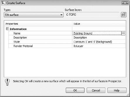
In Prospector, right-click the Surfaces branch and select Create Surface to display the Create Surface dialog.
Change the name to Existing Ground.
Verify that the style selected is Contours 1′ and 5′ (Background). You can also add a description during the surface creation, giving other users an idea of what that surface is representing. Your dialog should look like Figure 7.3. Click OK to close the dialog.
At this point, you've simply created the Existing Ground surface, but have not placed data in that surface definition. Remember that objects in and of themselves can be empty in Civil 3D, and it's the defining data that makes them powerful and dynamic.
Within Prospector, expand Surfaces → Existing Ground → Definition as shown in Figure 7.4.
Right-click the Contours branch and select Add to display the Add Contour Data dialog.
Click OK to accept the default values and dismiss the dialog.
Using a crossing window, select all of the entities in the drawing. The initial selection will include text and blocks as well as the intended polylines, but these will be weeded out.
Press Enter or right-click to complete the selection process, and the Existing Ground Surface will be built.
At this point, the surface is built purely from the polylines that described the contours in the original drawing. By adding the blocks representing items found by the survey crew, you can refine the surface and complete the topographic information for your site.
Under the Definition branch, right-click Drawing Objects and select Add to display the Add Points from Drawing Objects dialog.
Select Blocks from the drop-down menu in the dialog, and click OK.
Use a crossing window to again select the entire screen (there should be 32 objects selected).
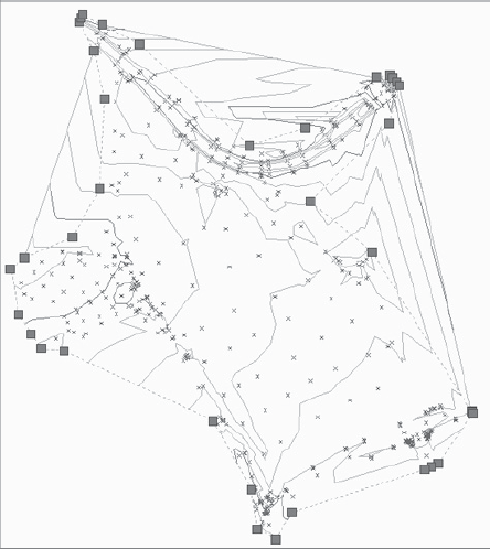
Press Enter or right-click to complete the selection process. The surface will rebuild, taking into account the new data, and your results should look similar to Figure 7.5. This is a good method for reproducing existing drawing files.
Close the drawing.


Because the blocks added to this surface were already quite close to the contour-generated surface, there's not much visual change reflected back to the display screen, but there has been a change in the underlying object. Although this method generally reflects the input data very well, it still is not as accurate as a surface built from field data. The next section deals with that issue.
The best way to understand existing conditions on a site is to visit it with a survey crew. This allows for human inspection of all the conditions and allows a trained professional to pick up all the data to represent the site correctly in a computer model. Based on points and often field-created linework, this type of surface is the ideal starting point for engineering work, and should be a requirement whenever practical. In the following exercise, you'll walk through adding surveyed points into a surface definition, and then adding breakline data to force the surface triangulation along certain lines:
Open the
Building from the Points.dwgfile.In the Prospector expand the Surfaces → Existing Ground → Definition branch.
Right-click the Point Groups branch and select Add to display the Add Point group dialog.
Select Field Survey from the list, and then click OK to close the dialog and build the surface.
At this point, the data is correct in general, but there are still some pretty significant errors you can fix by simply using the linework provided to create breaklines.
Within the drawing window, select one of the white polylines running along the edges of your site. These are lines created by the survey crew during their data-import process to define some site definition lines.
Right-click and select Select Similar to highlight the rest of the polylines on your site.
Without deselecting, right-click the Breaklines branch under the Existing Ground definition and select Add to display the Add Breaklines dialog.
Type Field Data into the Description blank, and click OK to complete the data addition and rebuild the surface.
The Panorama palette appears, giving a list of points that are duplicates. Because the vertices on the polylines just added match the point data, this is expected. Click the green check box to close Panorama and review the surface. It should look like Figure 7.6.
Close the drawing.
You've now built the same site in a number of different ways. Each method adds a level of accuracy, but each method adds a level of cost as well. When working with surface information, it's important to weigh the benefits of field survey information against the cost of a crew and decide accordingly on how you'll be building your site surfaces. Now that we've built a good surface, let's use a few more surface tools and edits to refine your existing ground model.

If you stop working with your surface after adding points and breaklines, you'll probably leave some inaccuracies in the model. There are a number of things you can do to refine a surface in Civil 3D, but because this book is introductory, we're going to examine only the two most common edits. First, you'll use a boundary to control triangulation across areas where you have little data, and then you'll tell Civil 3D to ignore the occasional blown shot.
There are a number of reasons to use boundaries when building surfaces. The obvious use (and the one covered in this section) is to limit the location of data and the triangles that connect the surface. Other uses can be to divide a surface along a phase line, to hide a building pad from surface analysis, or to show interior surface data that might be considered an island (such as the landscape inside a courtyard). Because the most common use is to limit data based on location, that's what you do in the following exercise:
Open the
Surface Boundary.dwgfile. This is the same surface you just built, but the point labels and breaklines have been turned off for clarity. Look at the areas indicated in Figure 7.7 and notice how contours appear in areas where you have very little point information.From the Modify tab and Ground Data panel on the ribbon, select Surface. A contextual tab called Surface will appear. From the Surface Tools panel, select Extract Objects to display the Extract Objects from Surface dialog.
Uncheck the Major Contour and Minor Contour check boxes and click OK to close the dialog. This utility creates a 3D polyline around the existing surface definition that you can use to refine and reapply a boundary.
Select the outside edge of the surface, and you should see a polyline highlight as in Figure 7.8.
Use AutoCAD editing techniques to manipulate this polyline until it looks similar to Figure 7.9. This indicates the desired outer limits of your surface. Notice that the polyline dips into the surface in the problem areas indicated previously in Figure 7.7.
In Prospector, expand the Surface Boundary drawing and the Surfaces Existing Ground-Definition branch.
Right-click the Boundaries branch and select Add to display the Add Boundaries dialog.
Uncheck the option for Non-destructive Breakline, and then click OK to accept the other values and dismiss the dialog.
Select the polyline you just modified, and Civil 3D will rebuild the surface, limiting the surface as specified.
Your surface should look something like Figure 7.10. Note that the surface boundary does not follow your polyline. The option you unchecked created a destructive breakline, ensuring that only data wholly contained in the boundary is part of the surface.
Close the drawing.


With a boundary in place, we'll now look at weeding out some bogus data. It's very common for surveyors to place points in a file that lay out the metes and bounds of a site, but have no vertical data. If you're not careful, those points sometimes slip into the surface definition and cause the surface to shoot down to a zero elevation at those locations. In the following exercise, you'll look at some easy options you can use as part of the Surface Properties to make filtering out bad data an automatic process:
Open the
Edit Surfacedrawing file. It's important to open this one instead of continuing with the previous file, because we've put some of the bad data back in the file for learning purposes. Notice that there seems to be some deep holes along the boundary, indicated by the large cluster of contours at those locations.From Prospector, expand the drawing and the surfaces branch.
Right-click the Existing Ground surface and select Surface Properties.
Switch to the Definition tab as shown in Figure 7.11.
Expand the Build options as shown in Figure 7.11 and change the Exclude Elevations Less Than value to Yes.
Change the Elevation < value to 100 and click OK to close the dialog. Civil 3D displays a warning that the surface needs to be rebuilt.
Click the Rebuild the Surface option to close the warning. Civil 3D updates the surface, recontouring the areas where zero elevations were affecting the model.
Close the drawing.

Although this simple edit handles a lot of situations, there are also tools for handling points that are too high, triangulating legs that are too long to be accurate, and reordering the build operations within the surface definition itself. As you work with surfaces and want to refine your output to a higher level, you should look at the automated tools in the Surface Properties Definition tab to make your job easier and faster.
You've created a number of different surfaces. Now let's consider the wide variety of display and labeling options.
Building surface models is one of the more satisfying tasks in Civil 3D. It's quick, it's easy to see an immediate return, and there are lots of interesting tools and settings. After you're done playing though, you need to share your model, and in most cases, that means printing. A good printout needs good labels, and because you have different print requirements, you'll wind up creating a number of different contours and a bunch of different labels to match—and that means a lot of work. Or does it?
Civil 3D's dynamic model makes it extremely easy to label contours, critical spots, and slopes along a surface model. In this section, we'll look at all three tasks.
As discussed in Chapter 1, all labels in Civil 3D are based on styles, and contours are no different. Remember that labels reflect the object itself and are dynamically related, so as you lay out your labeling, you can do so with confidence knowing that any future change will be accommodated by the label with no work on your part. Let's first look at labeling the ground surface you've been working with so far.
Open the
Contour Labels.dwgfile.From the Annotate tab and Labels & Tables panel on the ribbon, select Add Labels → Surface → Contour – Multiple at Interval.
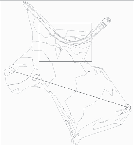
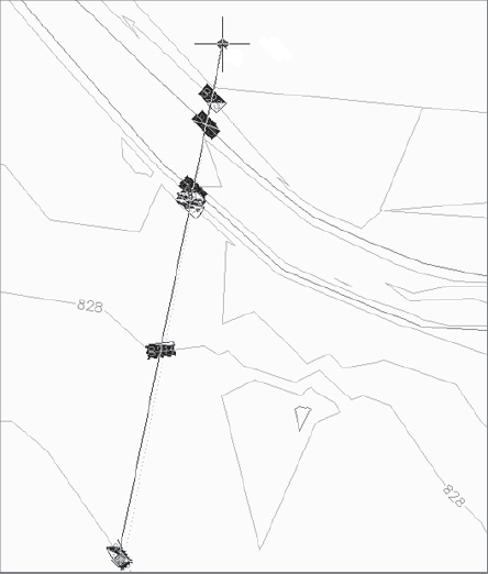
Using a center osnap, draw a line between the two circles on the screen, as shown in Figure 7.12.
Enter 300 at the command line to set the interval value of 300′. This will create a label 300′ along every contour, measured along the contour from the point of contour and the contour label line just drawn.
Although this labels a large portion of the site, it only labels the contours that the original line crosses, leaving some areas unlabeled. You could repeat the process, but it's often more efficient to use the labels placed by the first pass to create labels for the other areas.
Zoom in on the area indicated by the rectangle in the drawing and in Figure 7.12.
Select the 829 label. Notice that three grips appear, not one as you might expect. The label is actually a function of a contour label line. Every place this line crosses a contour, a label will be inserted.
Grab the northeastern-most grip of the three, and drag it to an approximate position as shown in Figure 7.13. Note the shadow box areas indicating where new labels will be placed on the surface.
Click to finalize the placement, and press Esc to deselect the label line.
Repeat steps 6, 7, and 8 with the other labels in the rectangle (828 elevations) and adjust them as desired. After a little grip editing, you should wind up with something similar to Figure 7.14.
Select one of the lines to highlight it, and then right-click and select Select Similar. This will select all of the contour label lines in the drawing file.
Right-click again and select Properties to display the AutoCAD Properties palette.
Within the Properties palette, change the Display Contour Label Line value to False as shown in Figure 7.15. Close the palette if you like.
Press Esc again to deselect the Contour Label Lines, and notice that the linework disappears but the labels do not.
Close the drawing.

With the labels in place, and the linework gone, you can plot or present this data as needed in other drawing files. Remember that you can get the Contour Label Line grips back by selecting any label. With the label selected, a visit to the Properties window will allow you to modify, change, or toggle the display of the labels and styles. Now that you have labeled the contours, you'll label some critical points on your surface.

The contours themselves are handy for getting a general feel for site information, but when you get down to it, there are critical points on every site where you must know the precise elevation. This could be a tie-in point, the top of a wall, or the elevation at a loading dock. In every case, this was generally considered tedious work, as any change to the design necessitated removing all those labels and starting over. Thankfully, Civil 3D's dynamic model lets you label once and update many times. In the following exercise, you'll quickly place a number of labels just to get a feel for the process and how these labels can be moved but retain the dynamic link to the surface being labeled:
Open the
Spot Labels.dwgfile.From the Annotate tab and Labels & Tables panel, select Add Labels → Surface Spot Elevation.
Turn on your center osnap and place labels in the four circles found in the drawing. Press the spacebar or Enter to exit the command.
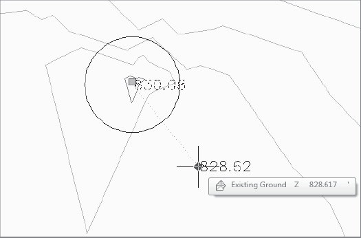
Zoom in on the northernmost circle and its label.
Select the label to show the two grips available for surface spot labels.
Click the diamond grip to relocate the label and begin dragging it as shown in Figure 7.16. Note that the label is updated on the fly as the label is dragged.
Press Esc to deselect the label and return it to its prior position.
Placing spot labels is quick, easy, and convenient. Now that you know about contours and specific locations, you'll use labels to get some more information about the site in general by labeling slopes in areas of interest.
When labeling slopes on a surface, it's important to remember that there are two ways of measuring the slope: at a single point based on the slope of the TIN triangle beneath that point, or between two points based on the distance and difference in elevation between those two points. Let's look at both methods of labeling.
Open the
Slope Labels.dwgfile.From the Annotate tab and Labels & Tables pallete on the ribbon, select Add Labels → Surface → Slope.
Press Enter at the command line to accept the default slope label type of one-point.
Using a center snap, place labels at the center of the four larger circles in the drawing. Press the spacebar or Enter to exit the command.
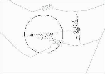
Zoom in on the red circle in the northeast portion of the site and the nearby label as shown in Figure 7.17. Note that because of the nature of the one-point label, the slope label and arrow are pointing in a direction that really doesn't make sense, parallel to the contours. One-point slope labels reflect the instant grade of a TIN triangle, sometimes leading to labeling anomalies like this one.
Select the label to display its one grip. Select the grip and begin to drag it away as shown in Figure 7.18. Note that the rotation and label text change as the insertion point moves across the surface.
Place the label in the center of the green circle just to the northwest. Move or replace the other labels as necessary.
This type of review is crucial in both methods of labeling slope. The main issue with the two-point label style is that it is possible to miss high or low points.
Zoom extents to bring the entire site back on-screen.
Select the slope again as in step 2.
Enter T at the command line to choose a two-point label style.
Using a center snap, pick one of the smaller circles on the north end of the site, and then pick the other small circle to the south, as shown in Figure 7.19.
Using the same center snap, connect the final two smaller circles with one more slope label. Using the longer span between points can help you understand the overall site conditions and prepare for drainage design.
Close the drawing.

With the surface labeled in a number of different ways, you have a good surface model that you can share with the team and use in plans or further analysis. In the next section, we'll look at analysis tools—reviewing the site on the front end for use suitability, and then performing an earthwork analysis with color-coded areas and soil adjustments.

A good model makes for easy plans, but being able to do more than just create nice linework is what makes Civil 3D so powerful. Two common tasks in land development are reviewing the interaction of a flood plain with a site, and understanding how much soil volume exists between existing and proposed conditions. Let's look at those tasks now.
Quite commonly, a consultant will be engaged to review a site for the suitability of a design based on site conditions. As metropolitan areas become more and more developed, the number of sites with floodplain areas increases. Understanding the interaction of this floodplain water elevation with the existing conditions helps engineers and developers make good site selection choices. In the following exercise, you'll take a look at coloring the surface based on elevation data:
Select the surface and right-click to display the shortcut menu.
Select Surface Properties to display the Surface Properties dialog.
On the Information tab, change the Surface Style to Elevation Banding (2D) as shown in Figure 7.20.
Switch to the Analysis tab.

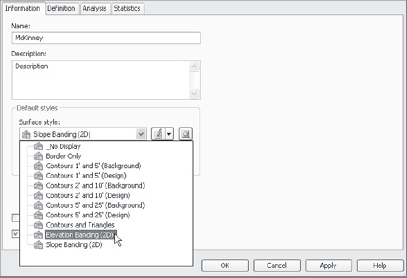
Figure 7.20. Selecting the Elevation Banding (2D) style turns on the display component for Elevations in plan view.
When you run the analysis with the stock values, Civil 3D will divide the range of surface elevation into a number of ranges, and assign colors based on a scheme determined by the style—Elevation Banding (2D) in this case. Because you need a more specific answer, you'll now manually tweak the ranges and colors to make more sense.
Based on information from your floodplain expert, the creek in this area has the following range of elevations:
Normal Creek Surface: 556.5
Flood Surface: 562
Minimum Freeboard Surface: 563.5
You'll use these elevations to drive your elevation analysis.
In the Range Details area of the dialog, click in the column of Maximum Elevation for the row marked 1 and enter 556.5 for a value.
Double-click the color block on row 1 to display the Select Color dialog. Select blue and click OK to close the dialog.
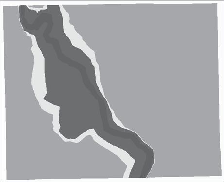
Continue working through the Minimum and Maximum elevations as shown in Figure 7.21, assigning colors as you go. The colors from top to bottom should be blue, red, yellow, and green.
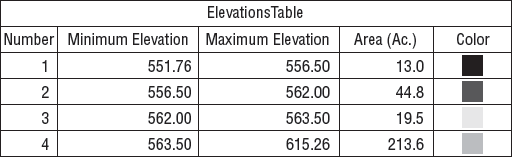
Click OK to close the dialog, and your screen should look like a rainbow of colors as shown (approximately) in Figure 7.22.
Although the colors are great, and give a very good visual feel for the land available for development, a legend table will complete the presentation, and is simple to add.
From the Annotation tab and Labels & Tables panel on the ribbon, select Add Tables → Add Surface Legend Table.
Press Enter at the command line to accept the default Elevations table type.
Press Enter to accept the default behavior of a dynamic table.
Select a location for the upper-left corner of your table and click.
Your table should look like Figure 7.23, and you're done with your analysis of the floodplain.
Close the drawing.

This type of cursory analysis tool, combined with the information available from Google Earth and local government data, means you can do site analysis in almost no time. Now, let's look at the other end of the project, and run some earthwork calculations.
As land-development projects near their final design stages, the amount of earthmoving always becomes a major design constraint. With Civil 3D's built-in analysis tool and volume surface tool, it's easy to review the design as it is and prepare earthworks calculations.
Open the
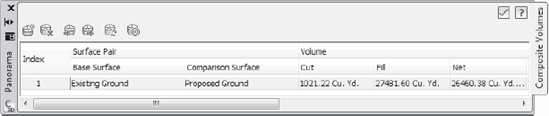
Earthwork Analysis.dwgfile. This drawing contains both the existing and proposed grade surfaces for the purpose of our sample.From the Analyze tab and Volumes and Materials panel on the ribbon, select Volumes → Volumes to display the Composite Volumes palette in Panorama.

Click the <Select Surface> drop-down list under Base Surface and select Existing Ground from the drop-down menu.
Click the <Select Surface> drop-down list under Comparison Surface and select Proposed Ground. As soon as you select the second surface, Civil 3D will complete a volume calculation and display the results within the palette as shown in Figure 7.24.
If you have information from a soils professional, you can also apply Cut and Fill factors by entering them manually here. You then need to reprocess the analysis to get updated results, which you'll do in a later step. But first, because the current result is approximately 26,000 yards of fill, you'll adjust the surface, and see how easy it is to get a new number.
Without closing Panorama, expand the Surfaces → Proposed Ground → Definition branch in Prospector.
Right-click the Edits option and select Raise/Lower Surface.
Enter −1 at the command line and press Enter. This moves the entire surface down one foot. Remember that this type of adjustment works while in the rough grading stages, but would be impractical later in the design.
Move back to Panorama, and click the Recompute Volumes button (the second button from the right). Your Composite Volumes should now resemble Figure 7.25, with a net volume near 8,600 cubic yards of fill.

Although the calculation here is quick and easy, it's unfortunately limited in that it disappears as soon as you close the Panorama palette. To create a more permanent volume calculation, it's necessary to create a TIN Volume Surface.
Close Panorama if you have not already done so.
Right-click Surfaces in Prospector, and select Create Surface to display the Create Surface dialog.
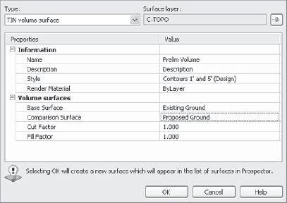
In the upper-left corner, click the Type: drop-down list and select the TIN Volume Surface option.
Change the Name value to Prelim Volume.
Verify that the Style is set to Contours 1′ and 5′ (Design).
Click the <Base Surface> cell, and then click the ellipsis button to display the Select Base Surface dialog.
Select Existing Ground, and click OK to dismiss the Select Base Surface dialog.
Click the <Comparison Surface> cell, and then click the ellipsis button to display the Select Comparison Surface dialog.
Select Proposed Ground and then click OK to dismiss the Select Comparison Surface dialog. Your Create Surface dialog should now look like Figure 7.26. If you have Cut and Fill factors, input them here to use those factors in your analysis.
Click OK to close the Create Surface dialog and run the volume analysis.
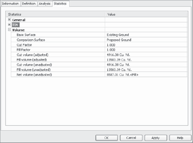
Back in the Prospector → Surfaces branch, right-click on the Prelim Volume surface that has now appeared and select Surface Properties to display the Surface Properties dialog.
Change to the Statistics tab and expand the Volume section as shown in Figure 7.27. Note that the Net Volume value is approximately 8,600 yards, exactly the same as with the other method.
Click OK to close the dialog.
With a TIN surface, you can now use the myriad of surface tools and labeling techniques to present the volume information in a concise manner. Think about using the elevation analysis to find the areas of most cut and fill, or the Spot Elevations on Grid option to create a map of cut-fill ticks.
Close the drawing.
Surfaces are major underlying components of a land development model. Creating them from a myriad of data sources allows you to represent most situations found in practice as a digital model with all the advantages that brings. Digital models and dynamic labels enable you to minimize rework during the plan production stage. Dynamic models and powerful analysis tools enable you to explore design alternatives and paths with less time spent going backward. By using even the basic portion of the Civil 3D surface modeling suite of tools, you're bound to cut hours from some of the most tedious tasks in land-development projects.