3Linear and Planar Array Factor Synthesis

The array factor is a function of the amplitude and phase weights, the relative element positions, and the frequency. Values for these variables exist that yield a desirable array factor (as long as the laws of physics are obeyed). This chapter presents analytical, statistical, and numerical techniques to synthesize or optimize an array factor.

3.1. SYNTHESIS OF AMPLITUDE AND PHASE TAPERS

The techniques presented in this section are more academic than practical. They provide some insight into the design of low-sidelobe tapers, but the fact that amplitude and phase weighting are required and that the weights can significantly vary from element to element make them very difficult to implement with real hardware.

3.1.1. Fourier Synthesis

In Chapter 2, the array weights were shown to be coefficients of a Fourier series. These coefficients come from the inner product of the desired array factor with a single Fourier component.

where m is one of the M harmonics. The number of elements in the array is 2M (even) or 2M + 1 (odd). Note that u ranges from −1 to +1. The limits on the integral should also span this range. Thus,

If d > λ/2, then the limits of integration do not cover the range of u. If d < λ/2, then the limits of integration cover a greater range than −1 to +1. Sine terms in the Fourier series expansion are included whenever the current weights (amplitude and phase) are not an even function with respect to the center of the array.

Equations (3.1) and (3.2) provide a method of synthesizing a desired array factor for a given number of elements. The steps needed in a Fourier synthesis technique are as follows:

1. Determine desired pattern AF(u).
2. Determine number of elements and element spacing.
3. Calculate limits of integration.
4. Find the w_m using (3.1) or (3.2).

Example. Design a 16-element equally spaced array to receive signals at a constant level over an angular range of –0.5 ≤ u ≤ 0.5 and zero elsewhere.

The specifications require that M = 8 and the array factor is represented by

The weights derived using the Fourier series synthesis method are shown in Figure 3.1 and the corresponding array factor in Figure 3.2. Some of the weights are negative, so the amplitude weights also have to be accompanied by 180° phase shifts.

The amplitude taper for low sidelobes in a sum pattern will not result in the same low sidelobes in a difference pattern and vice versa. Since the difference array factor is an odd function, the weights for a difference array are the inner product of the desired array factor with a single Fourier sine component.

Example. Find the weights for a 20-element array with a difference pattern having the following specifications:

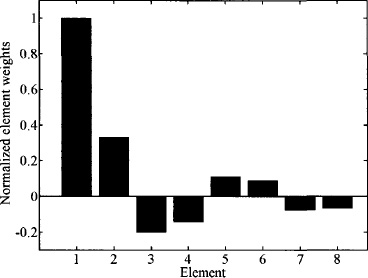
Figure 3.1. Fourier coefficients or array weights for the 16-element array.

Figure 3.2. Array factor corresponding to the Fourier coefficients.

Substituting into (3.4) and solving yields

Figure 3.3. Fourier coefficients or array weights for the 16-element difference array.

w = [−0.0124   −0.0836   −0.0988    −0.0207   −0.0266
−0.2170  −0.3620     −0.1860    0.1860  0.3620
   0.2170   0.0266  0.0207   0.0988 0.0836 0.0124]   

The weights derived using the Fourier series synthesis method are shown normalized in Figure 3.3 and the corresponding difference array factor in Figure 3.4.

3.1.2. Woodward–Lawson Synthesis

Sines and cosines are not the only building blocks that can be used to create array factors. An array factor is also the weighted sum of steered linear array factors [1,2].

where the coefficients are the samples of the desired array factor given by

The samples are taken at points where the maximum of one beam is at a zero of all the other beams (the beams are orthogonal).

Figure 3.4. Difference array factor corresponding to the Fourier coefficients.

Figure 3.5. Woodward–Lawson array weights for the 16-element array.

With this approach, the amplitude weights for the array are given by

Example. Repeat the Fourier series array synthesis example using the Woodward–Lawson synthesis technique.

Figure 3.5 is a plot of the resulting array weights and Figure 3.6 is the corresponding array factor with the beams and desired array factor superimposed.

Figure 3.6. Array factor corresponding to the Woodward–Lawson array weights.

3.1.3. Least Squares Synthesis

A more direct approach to array factor synthesis formulates the linear or planar array factor equation into a set of M equations with N unknowns. Samples of the desired array factor are taken at M points (AF₁, AF₂,…, AF_M) and form a column vector for the right-hand-side of a matrix equation.

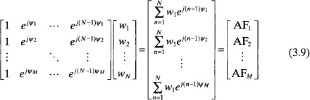
Each row in (3.9) is the array factor with the w_n as unknowns. If M = N, then the weights are found using a direct matrix inversion. Otherwise, a least squares solution is necessary to solve the over or under determined system of equations.

Example. Repeat the Fourier series and Woodward–Lawson example using a least squares approach.

Taking 20 equally spaced samples of the array factor for the right-hand-side vector permits a direct matrix inversion to find the array weights. and array factor are very similar to those of the previous examples, so the synthesized weights are compared to those of the Fourier series and Woodward–Lawson techniques in Table 3.1

TABLE 3.1. Amplitude Weights for Half of the Array Synthesized to Produce the Desired Array Factor for a 16-Element Array

Unlike Fourier and Woodward–Lawson synthesis methods, the least squares technique works for any element lattice and array shape. As with the other methods, the synthesized weights are complex and highly oscillatory. Also, the array factors are matched either exactly or in a least squares sense at M specified points. A much more desirable approach would be to place limits on the power pattern and the array weights. This can be done using a robust, global optimization technique like a genetic algorithm. Many examples of optimizing array factors using a genetic algorithm may be found in the literature [3,4].

3.2. ANALYTICAL SYNTHESIS OF AMPLITUDE TAPERS

There are many different methods to synthesize amplitude weights that produce desirable sidelobe levels. This section presents several approaches to analytically calculate the array weights for linear and planar arrays. In general, the analystical synthesis approaches require linear or circular apertures. Weights for all other geometries must be numerically found.

3.2.1. Binomial Taper

If all the unit circle zeros of an array factor are at ψ = 180°, then the array factor has no sidelobes and is written as

TABLE 3.2. List of Binomial Amplitude Weights for Arrays with 1 through 9 Elements

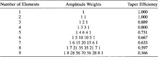
Figure 3.7. Array factors normalized to the number of elements in the array for several sizes of binomial arrays.

The corresponding amplitude weights are the binomial coefficients, hence this array is known as a binomial array [5]. Table 3.2 lists the binomial coefficients for up to nine element arrays, and Figure 3.7 shows some examples of binomial array factors normalized to a uniform array factor of the same size. The taper efficiency for binomial arrays is very low. The price paid for lowering sidelobe levels is a decrease in taper efficiency (Table 3.2) and directivity and a corresponding wide main beam. Errors are always present in an array, so even though the amplitude taper results in no sidelobes, the array factor has error sidelobes. Consequently, other more efficient sidelobe tapers with sidelobe levels comparable to the error sidelobes are more desirable.

3.2.2. Dolph–Chebyshev Taper

Rather than totally eliminating the sidelobes by using the binomial coefficients as the array weights, sidelobe levels can be set to a specified level by mapping the array factor to a Chebyshev polynomial [6]. The Chebyshev polynomials are represented by

When x is between one and minus one, these polynomials oscillate as a cosine function with a maximum amplitude of one (for m = 0, 1, …, 4 graphed in Figure 3.8). Outside of that range, they quickly increase or decrease as described by the cosh function in (3.11).

Assume the maximum sidelobe level is 1.0, so that it equals the height of the ripples of the Chebyshev polynomial between −1 ≤ x ≤ 1. The number of sidelobes corresponds to the number of extrema in the polynomial. An N element array corresponds to a Chebyshev polynomial of order N – l. If the sidelobes are to be sll (in dB) below the peak of the main beam, then the value of the Chebyshev polynomial at the peak of the main beam must equal

Setting (3.11) equal to (3.12) results in the peak of the main beam at

Figure 3.8. Graph of the first four Chebyshev polynomials for 0 ≤ m ≤ 4.

where

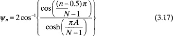
Now, the main beam maps to the Chebyshev polynomial. Next, the array factor zeros (nulls) map to the zeros of the Chebyshev polynomial. The zeros of the Chebyshev polynomial are located at

Mapping the zeros of the array factor to the zeros of the Chebyshev polynomial is done through the following relation:

The following equation provides the zeros of the array factor that correspond to a sidelobe level in dB of sll:

When the number of elements and sidelobe level are specified, the null locations on the unit circle are easily determined. Once the ψ_n are known, the polynomial in factored form easily follows. Multiplying all the factored terms results in a polynomial of degree N – 1. The polynomial coefficients are the amplitude weights for the array elements.

It turns out that for a specified sidelobe level, the Dolph–Chebyshev taper has the minimum null-to-null beam width. A reverse process is possible in which the lowest sidelobe level can be found for a specified null-to-null beamwidth [6]. The beam-broadening factor for a Chebyshev array is given by [7]

Figure 3.9 is a plot of taper efficiency as a function of sidelobe level for Chebyshev arrays having 10, 20, and 40 elements. Smaller arrays have a peak efficiency at a higher sidelobe level than do larger arrays. The peak efficiency of the smaller arrays is higher than the peak efficiency of the larger arrays. As the sidelobe level decreases, the taper efficiency of the larger arrays surpasses that of the smaller arrays.

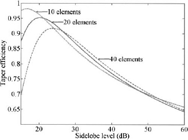
Figure 3.9. Taper efficiency versus sidelobe level for Chebyshev arrays.

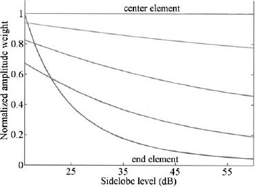
Figure 3.10. Normalized amplitude weights for a 10-element Chebyshev array versus sidelobe level.

Figure 3.10 are the normalized weights for a 10-element Chebyshev array as a function of sidelobe level. The end element does not have the smallest amplitude for sidelobe levels above –22 dB. At –22 dB and below, the weights monotonically decrease from the center to the edge. Similar behavior occurs for larger arrays too. The center amplitude weight for a 40-element array does not become larger than the edge element weight until the sidelobe level is –25 dB or below as shown in Figure 3.11.

Figure 3.11. Normalized center and end amplitude weights for a 40-element Chebyshev array versus sidelobe level.

Example. Design a 6-element array (d = 0.5λ) with –20-dB sidelobes.

First, find the ψ_n:

Next, write the polynomial in factored form:

Multiplying these factors together yields

The coefficients of AF are the amplitude weights for the 6-element array pattern in Figure 3.12 with η_T = 0.944.

Tseng and Cheng developed a Chebyshev synthesis technique for rectangular arrays with an equal number of elements in the x and y directions [8]. They applied the Baklanov transformation [9] to represent the array factor (a function of two angle variables: u and v) as a polynomial of one variable, t.

Figure 3.12. Array factor for a 6-element 20-dB Dolph–Chebyshev array.

With some manipulation, the weights for the fourth quadrant of a rectangular array are given by

for m, n = 1,2, …, N. The element spacing in the x and y directions can be different, but the number of elements in those directions must be the same.

Example. Calculate the Chebyshev weights for a 30-dB square array with 256 elements. Plot the array factor. The element spacing is square with d_x = d_y = 0.5λ.

The weights are calculated and shown in Figure 3.13. The array factor appears in Figure 3.14. The weights are real but do not monotonically decrease from the center to the edges.

3.2.3. Taylor Taper

The Chebyshev weighting is practical for a small linear array; but as N becomes large, the amplitude weights at the edge of the aperture increase. Increasing the edge taper presents problems with edge effects and mutual coupling. Other amplitude tapers are better suited for large, low-sidelobe arrays. One such taper was developed by Taylor [10]. The Taylor taper is a continuous taper for line sources that can be sampled for application to antenna arrays. The Taylor taper is similar to the Chebyshev taper in that the maximum sidelobe level can be specified. The difference is that the Taylor taper only has the first – 1 sidelobes on either side of the main beam at a specified height. All remaining sidelobes decrease at the same rate as the corresponding side-lobes in a uniform array.

Figure 3.13. Weights for the 30-dB square Tseng–Cheng–Chebyshev array with 256 elements arranged in a square grid having d_x = d_y = 0.5λ.

Figure 3.14. Array factor for the Tseng–Cheng–Chebyshev array.

The Taylor taper moves the first – 1 nulls on either side of the main beam away from the main beam. This equates to moving the corresponding zeros on the unit circle closer to the negative real axis. Since the other zeros remain untouched, the outer sidelobes and nulls stay in the same locations as those for a uniform array. The null locations for the Taylor array factor are calculated from

with A given by (3.14). These null locations translate to zeros on the unit circle by

Next, the factored form of AF is found. Multiplying the terms together gives a polynomial whose coefficients are the Taylor weights.

Example. Find the amplitude weights and array factor for a 20-element Taylor taper with – 5 and sidelobes 20 dB below the peak of the main beam.

A = 0.95                                                                
u_n = ±.117,±.193,±.291,±.394,±.5,±.6,±.7,±.8,±.9,1

Converting u_n into ψ_n produces

±0.367, ±0.607, ±0.914, ±1.239, ±1.571, ±1.885, ±2.199, ±2.513, ±2.827,3.142

and forming the polynomial equation yields

AF = 0.667z¹⁹ + 0.621z¹⁸ + 0.589z¹⁷ + 0.624z¹⁶ + 0.718z¹⁵ + 0.818z¹⁴
       + 0.888z¹³ + 0.933z¹² + 0.972z¹¹ + z¹⁰ + z⁹ + 0.972z⁸ + 0.933z⁷
              + 0.888z⁶ + 0.818z⁵ + 0.718z⁴ + 0.624z³ + 0.589z² + 0.621z + 0.667  

Figure 3.15 and Figure 3.16 show graphs of the amplitude weights and array factors, respectively. The efficiency is given by η_T = 0.965.

Notice that the first four sidelobes in Figure 3.16 slowly drop off rather than stay constant as expected. The peak sidelobe level is predicted accurately, though.

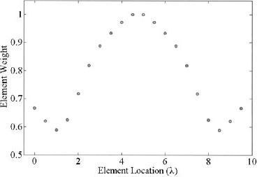
Figure 3.15. Amplitude weights for Taylor 20-dB, = 5 taper.

Figure 3.16. Array factor for Taylor 20-dB, = 5 taper.

The previous method of obtaining the Taylor amplitude weights is numerically inefficient for a large number of elements due to the many convolutions with the polynomial zeros to obtain the full polynomial. The weights become unsymmetrical for arrays larger than 50 elements. A more direct and numerically stable method is given by the formula

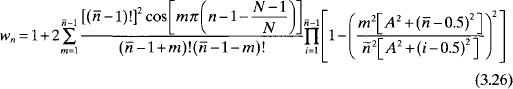
Figure 3.17. Plot of the that yields the most efficient taper for a given sidelobe level.

This formula is easy to program and finds the weights for very large linear arrays but becomes unstable for large values of . The formula in (3.26) can be used to calculate the taper up to a sidelobe level of 40 dB and = 81 using MATLAB. An above 86 requires higher precision and/or putting (3.26) in a format even less prone to numerical errors. It is recommended to compute the product in (3.26) using logarithms and then converting back by raising the result to the base.

For a specified sidelobe level, there is an that results in a maximum directivity. As increases, more energy goes into the sidelobes until a point is reached where the directivity decreases. As decreases, the beamwidth increases, so power is robbed from the peak of the main beam in order to increase the width of the main beam. The graph in Figure 3.17 indicates the (sidelobe levels between 15 and 45 dB) that results in the largest η_T. Although a large η_T is desirable, it is not the only consideration when implementing an amplitude taper. For small , the amplitude taper monotonically decreases from the center to the edge. Above a certain for a given sidelobe level, however, the amplitude taper increases at the edges. Consider the amplitude tapers for a 30dB Taylor taper with = 1 and = 23 shown in Figure 3.18. The = 7 amplitude taper is the most efficient taper while still having a monotonically decreasing amplitude from the center of the aperture to the edge. The = 23 taper has the highest efficiency. In most arrays, a monotonically decreasing amplitude taper is desirable, because the feed network is easier to build and the contribution from the edge elements are minimized. A plot of the that yields the most efficient taper for a given sidelobe level while still having a monotonically decreasing amplitude is shown in Figure 3.19. The needed for the most efficient taper dramatically increases as the sidelobe level decreases. In general, computing such a high is not necessary, since the monotonically decreasing tapers are more desirable and not that less efficient (see Figure 3.20).

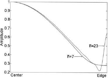
Figure 3.18. Taylor 30-dB amplitude tapers for = 7 and = 23.

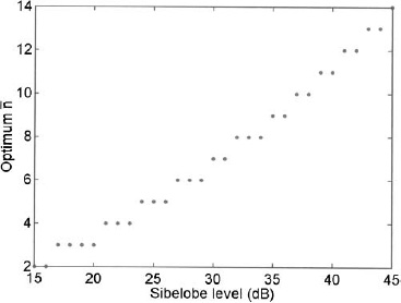
Figure 3.19. Plot of the that yields the highest η_T while still having a monotonically decreasing amplitude taper.

Taylor developed a similar taper for a desired sidelobe level without having to specify [11]. Weights for the one parameter taper are given by

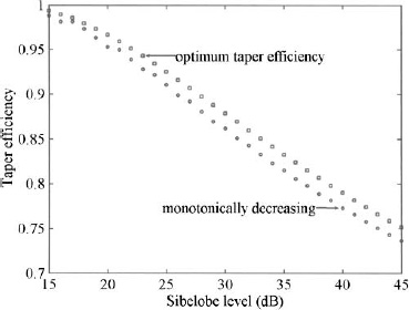
Figure 3.20. Graph of η_T versus sidelobe level for Taylor tapers that have an optimum η_T and the highest η_T while still having a monotonically decreasing amplitude taper.

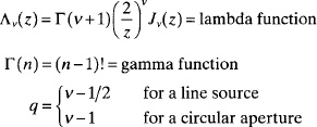
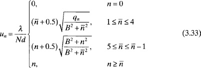
where I₀ is the zeroth-order modified Bessel function of the first kind, B is the Taylor parameter, is the distance of element from origin, and r_max is the array radius. The Taylor one parameter is related to the relative sidelobe level of the array and can be found by solving

where sll_dB is the maximum relative sidelobe level in decibels. Figure 3.21 is a plot of the efficiency at a particular sidelobe level for the Taylor one parameter taper. This taper is not as efficient as those displayed in Figure 3.20.

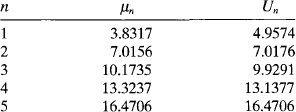
Taylor extended his amplitude taper for a continuous line source to a continuous circular aperture [12]. The following formula calculates the amplitude weights for a discrete Taylor taper for a circular aperture:

where is the distance from array center; r_max radius of circular array; J₁(μ_m) = 0, m = 1, …, ; μ_m = is the is the zeros of J₁; and . As with the continuous line source, samples of this taper are taken at the normalized element locations.

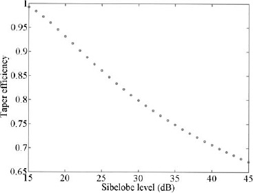
Figure 3.21. Efficiency versus sidelobe level for the Taylor one parameter amplitude taper.

Example. Calculate the 30-dB, = 5 Taylor weights for a circular array with 284 elements. Plot the array factor when the elements are on a square grid with d_x = d_y = 0.5λ.

First, calculate A = 1.32. Next, find the Bessel function zeros and the null movements.

Finally the weights are calculated and shown in Figure 3.22. Weight values are difficult to read from Figure 3.22, so a plot of the weights as a function of normalized distance from the center of the array is shown in Figure 3.23. The corresponding far field pattern is shown in Figure 3.24 with a cut in the = 0° plane shown in Figure 3.25.

It is possible to find the for a given sidelobe level that results in the highest taper efficiency while maintaining a monotonically decreasing amplitude taper (Figure 3.26). The previous example selected = 5 for a 30-dB sidelobe level. If = 4 were selected, then the dashed line in Figure 3.23 results. It has less area under the curve, so it is less efficient. If = 6 were selected, then the dotted line in Figure 3.23 results. Note that this taper is more efficient but is not monotonically decreasing. Figure 3.27 is a graph of the taper efficiency versus sidelobe level when the Taylor taper has the highest η_T while still having a monotonically decreasing amplitude taper.

Figure 3.22. Weights for the Taylor 30-dB, = 5 array with with 284 elements arranged in a square grid having d_x = d_y = 0.5λ.

Figure 3.23. Taylor 30-dB, = 5 weights.

Figure 3.24. Array factor for the weights in Figure 3.22.

Figure 3.25. Array factor as a function of θ for = 0°.

Hansen developed a low-sidelobe distribution for circular apertures that has a desired maximum sidelobe level and is specified by a single parameter [13]. His approach follows that of Taylor for the Taylor one-parameter taper. The amplitude distribution is given by

where H is the Hansen parameter found by solving

Figure 3.26. Plot of the that yields the highest η_T while still having a monotonically decreasing circular Taylor amplitude taper.

Figure 3.27. Graph of η_T versus sidelobe level for Taylor tapers that have the highest η_T while still having a monotonically decreasing amplitude taper.

and I₁ is the first-order modified Bessel function of the first kind.

Example. Calculate the 30-dB Hansen one-parameter weights for a circular array with 284 elements. Plot the array factor. The square element lattice has d_x = d_y = 0.5λ.

Figure 3.28. Weights for the 30-dB Hansen one-parameter array with with 284 elements arranged in a square grid having d_x = d_y = 0.5λ.

Figure 3.29. The 30-dB Hansen one-parameter weights.

First, find H = 1.1977. Next, the weights are calculated and shown in Figure 3.28. Weight values are difficult to read from Figure 3.28, so a plot of the weights as a function of normalized distance from the center of the array is shown in Figure 3.29. The corresponding far field pattern is shown in Figure 3.30 with a cut in the = 0° plane shown in Figure 3.31.

Figure 3.30. Array factor for the weights in Figure 3.28.

Figure 3.31. Array factor as a function of θ for = 0°

Figure 3.32 is a graph of the efficiency versus sidelobe level for the Hansen one-parameter amplitude taper. In general, the sidelobe levels drop off dramatically which produces a much less efficient Taper than is possible with the Taylor weights.

Figure 3.32. Efficiency versus sidelobe level for the Hansen one-parameter amplitude taper.

3.2.4. Bickmore–Spellmire Taper

The Bickmore–Spellmire taper for a linear or circular array encompasses some of the amplitude tapers already covered and can be written as [14]

Where

with A given by (14). Two special cases of interest occur when v = 1/2 (Taylor’s one-parameter) and v = 1 (Hansen’s one-parameter). For a given v, A can be varied to effect a tradeoff between beamwidth and peak sidelobe level. Picking A holds the beamwidth constant, so v governs a tradeoff between the peak sidelobe level near the main beam and the height of the more remote sidelobes.

3.2.5. Bayliss Taper

Bayliss developed a low sidelobe taper for difference patterns that is analogous to the Taylor taper for sum patterns [15]. The Bayliss taper has – 1 equally high sidelobes on either side of the main beam, while the rest decrease away from the main beam as with a uniform difference pattern. Null locations are given by

where

The peak of the difference array factor is located at

Example. Find the amplitude weights and array factor for a 20-element Bayliss taper with = 5 and –20-dB sidelobes.

B = 0.95                                                                   
u_n = ±.117,±.193,±.291,±.394,±.5,±.6,±.7,±.8,±.9,1

Converting u_n into ψ_n produces

±0.367, ±0.607, ±0.914, ±1.239, ±1.571, ±1.885, ±2.199, ±2.513, ±2.827,3.142

Figure 3.33. Bayliss amplitude weights

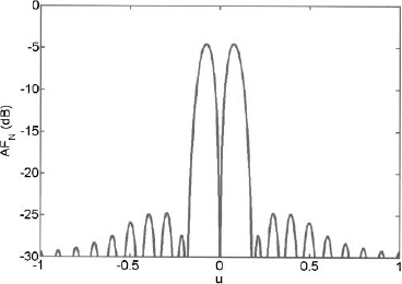
Figure 3.34. Bayliss 20-element array factor.

and forming the polynomial equation yields

AF = 0.667z¹⁹ + 0.621z¹⁸ + 0.589z¹⁷ + 0.624z¹⁶ + 0.718z¹⁵ + 0.818z¹⁴
       + 0.888z¹³ + 0.933z¹² + 0.972z¹¹ + z¹⁰ − z⁹ − 0.972z⁸ − 0.933z⁷
         − 0.888z⁶ − 0.818z⁵ − 0.718z⁴ − 0.624z³ − 0.589z² − 0.621z − 0.667             

The resulting amplitude weights and array factor are shown in Figures 3.33 and 3.34.

In the same paper, Bayliss developed his taper for a circular difference array by moving the zeros of the first-order Bessel function. Half of the aperture receives a 180° phase shift. The weights are given by the formula

Where

with A given by (3.14). The cos term forces the weights in half of the aperture (x < 0) to be negative. The null occurs at = 90° or 270° for all θ.

Example. Calculate the 30-dB = 5 Bayliss weights for a circular array with 284 elements. Plot the array factor. The element spacing is square with d_x = d_y = 0.5λ.

First, calculate A = 1.32. Next, find the zeros of J₁(r) and the null movements.

Finally, the weights are calculated and shown in Figure 3.35. Weight values are difficult to read from Figure 3.35, so a plot of the weights as a function of normalized distance from the center of the array is shown in Figure 3.36. The corresponding far field pattern is shown in Figure 3.37 with a cut in the = 0° plane shown in Figure 3.38.

3.2.6. Unit Circle Synthesis of Arbitrary Linear Array Factors

Sometimes the standard amplitude tapers are not sufficient to meet design specifications. This section presents several examples of using the unit circle to create desirable linear array factors [16]. The consequence of most of these designs is that the element weights are complex rather than real. If each array polynomial root has a complex conjugate pair, then the weights are real.

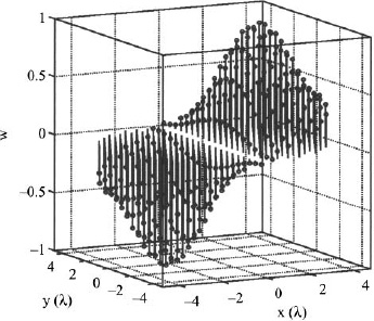
Figure 3.35. Weights for the 30-dB, = 5 Bayliss array with with 284 elements arranged in a square grid having d_x = d_y = 0.5λ.

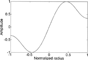
Figure 3.36. Bayliss 30-dB, = 5 weights.

Otherwise, they are complex. Elliot presents numerous examples of synthesizing modified Taylor patterns and null free array factors in his book [17]. These topics are presented as examples here. Their practical value is limited and numerical synthesis methods provide superior results today.

Example. In this example, very low sidelobes are needed for u < 0 while only low sidelobes are needed for u > 0. The desired array factor has the following characteristics:

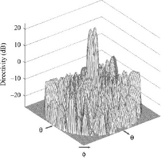
Figure 3.37. Array factor for the weights in Figure 3.35.

Figure 3.38. Array factor as a function of θ for = 0°.

1. Taylor = 5 sll = 25 dB for u < 0.
2. Taylor = 3 sll = 15 dB for u > 0.

This is a two-step process. First, the roots are found for the 25-dB taper and the 15-dB taper. Next, only the roots from the 15-dB taper that have an imaginary part less than zero are kept, then the roots from the 25-dB taper that have an imaginary part greater than or equal to zero are kept. These roots are then placed in factored form and multiplied to get the array polynomial. The complex weights of this polynomial are the weights shown in Figure 3.39. The corresponding unit circle is in Figure 3.40 and the array factor in Figure 3.41.

Figure 3.39. Synthesized amplitude weights (solid line) and phase weights (dashed line).

Figure 3.40. Unit circle of asymmetrical Taylor weights.

Example. Start with a Taylor = 4 sll = 25-dB taper and place a null at u = 0.25 when d = 0.5λ. Do not allow complex weights.

First, the roots of the Taylor taper are found:

Figure 3.41. Array factor of asymmetrical Taylor weights.

Figure 3.42. Unit circle representation of the initial Taylor taper and the null at u = 0.25.

−1.0000, −0.9509 ± j0.3094, −0.8085 ± j0.5885, −0.5867 ± j0.8098, −0.3072 ±
j0.9516, 0.0026 ± j1.0000, 0.3124 ± j0.9499, 0.5977 ± j0.8017, 0.8092 ± j0.5875,
0.9066 ± j0.4220

For a null at u = 0.25, r_null = cos(.25kd) + jsin(.25 kd) = 0.7071 + j0.7071.

To keep the weights real, then the roots should be complex conjugate pairs. Replace the roots 0.8092 ± j0.5875 with the roots 0.7071 ± j0.7071. The new roots are shown on the unit circle in Figure 3.42. Weights from the Taylor taper and the nulled taper are in Figure 3.43. The two array factors are shown in Figure 3.44.

Figure 3.43. Amplitude weights for the Taylor taper and the null at u = 0.25.

Figure 3.44. Array factor for the Taylor taper and the null at u = 0.25.

Example. Modify a 20-element uniform array with d = 0.5λ so that it has a flat top from −0.1 < u < 0.1 and sidelobes 20 dB below the main beam.

This problem could be done best using numerical methods. Here, a good guess is used instead. A zero placed on the real axis and outside the unit circle in order to flatten the main beam. Also, the first two zeros on either side of the main beam are removed to give the main beam room to expand. Adding one zero and removing 4 zeros while maintaining d = 0.5λ necessitates that there are only 17 elements in the new array. The resulting weights are

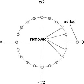
Figure 3.45. Unit circle representation for the flat top main beam and uniform arrays.

w = [0.026  0.081  0.144  0.174  0.132  −0.003  −0.224  −0.493  −0.750
       −0.934  −1.0  −0.936  −0.766  −0.539  −0.314  −0.139  −0.037]

The uniform array and the flat top main beam array are compared via the unit circle (Figure 3.45), the amplitude weights (Figure 3.46), and the array factors (Figure 3.47).

3.2.7. Partially Tapered Arrays

A partial array taper uses only a subset of all the element weights to control the array factor [18]. Center elements have an amplitude of 1 and a phase of 0. Edge element weights are synthesized using an appropriate numerical method. The partially tapered array factor is

where N_cen is the number of uniformly weighted elements in the center and N₁ and N₂ are the number of weighted edge elements. The center Fourier coefficients are all one. If the array has an even number of equally spaced elements and is symmetric about the center of the array, then N₁ = N₂ = (N − N_cen)/2 and the array factor is written as

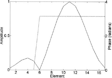
Figure 3.46. Amplitude (solid line) and phase (dashed line) weights for the flat top main beam array.

Figure 3.47. Array factors for the flat top main beam and uniform arrays.

Equation (3.38) may be rewritten in matrix form

The weights in (3.39) can be found using least squares described earlier or one of the numerical methods described in the next section.

3.3. NUMERICAL SYNTHESIS OF LOW-SIDELOBE TAPERS

Analytical approaches to finding optimum array amplitude weights are still used today. They work well because the unknown array weights are coefficients of a complex Fourier series. If the unknowns are the element spacings or element phases, then they appear in the complex exponent and are not easily found. Checking all combinations of values of the array variables is not realistic unless the number of variables is small. Optimizing one variable at a time does not work nearly as well as following the gradient vector downhill. The steepest descent method, invented in the 1800s, is based on this concept and is still widely used today [19]. Newton’s method uses second-derivative information in the form of the Hessian matrix to find the minimum. Although more powerful than steepest descent, calculating the second derivative of the cost function may be too difficult.

In order to avoid the calculation of derivatives, Nelder and Mead introduced the downhill simplex method in 1965 [20]. This technique has become widely used by commercial computing software like MATLAB because it is very stable. A simplex has n + 1 sides in n-dimensional space. Each iteration generates a new vertex for the simplex. A new point replaces the worst vertex when it is better. In this way the simplex gets smaller and the solution becomes more accurate.

Successive line minimization methods were developed in the 1960s [21]. A successive line minimization algorithm starts at a random point and then moves in a predetermined direction until the cost function increases. Then, it tries a new direction. A conjugate direction does not interfere with the minimization of the prior direction. Powell developed a technique in which changes to the gradient of the cost function remain perpendicular to the previous conjugate directions [22]. The BFGS algorithm [23-26] approximates the Hessian matrix (square matrix of second-order partial derivatives) in order to calculate the next search point. This algorithm is “quasi-Newton” in that it is equivalent to Newton’s method for prescribing the next best point to use for the iteration, yet it doesn’t use an exact Hessian matrix. Quadratic programming is a technique that assumes that the cost function is quadratic (variables are squared) and that the constraints are linear. It is based upon Lagrange multipliers and requires derivatives or approximations to derivatives [19].

Numerical optimization has been used to find nonuniform element spacings, complex weights, and phase tapers that resulted in desired antenna patterns. Some examples of nonuniform spacing synthesis include dynamic programming [27], Nelder Mead downhill simplex algorithm [28], steepest descent [29], and simulated annealing [30]. Numerical methods were used to iteratively shape the main beam while constraining sidelobe levels for planar arrays [31-33]. Linear programming [34] and the Fletcher–Powell method [35] were applied to optimizing the footprint pattern of a satellite planar array antenna. Quadratic programming was used to optimize aperture tapers for various planar array configurations [36,37]. Numerical optimization was used to find phase tapers that maximized the array directivity [38], and a steepest descent algorithm was used to find the optimum phase taper to minimize sidelobe levels [39].

The cost function returns the values of an attribute of an array antenna that are to be minimized. As an example, consider finding the minimum maximum sidelobe level of a 6-element array by adjusting either the amplitude weights, element spacing, or phase weights of a linear array that lies along the x axis [40]. The spacing, amplitude weights, and phase weights are symmetric with respect to the center of the array, so only the right half of the array needs to be specified. In order to visualize the cost surface, only two variables can be used. The center two elements have an amplitude of one and a phase of zero. Figure 3.48 is the cost function when the amplitude weights are the optimization variables with limits 0.1 ≤ a_2,3 ≤ 1.0, and δ_1,2 = 0 and x₁ = 0.25λ, x₂ = 0.75λ, and x₃ = 1.25λ. Figure 3.49 is the cost function when a_2,3 = 1.0, 0 ≤ δ_1,2 ≤ π, and x₁ = 0.25λ, x₂ = 0.75λ, and x₃ = 1.25λ. Figure 3.50 is the cost function when a_2,3 = 1.0 and δ_1,2 = 0, and the element spacings are bound by x₁ = 0.25λ, x₂ = 0.25λ + Δ₂, and x₃ = 0.25λ + Δ₂ + Δ₃.

All the cost functions in these figures have ridges, narrow valleys, and dramatic variations in slope. The cost surface variations slows the convergence of local minimization algorithms. Speed of convergence and quality of the minimum depends upon the starting point. For the 6-element case, the local minimization algorithms find the true minimum most of the time. On the other hand, adding more array variables increases the cost surface complexity by introducing many other local minima that fool local optimizers.

Figure 3.51 is a graph of the maximum sidelobe level in decibels versus the thinning configuration for a 32-element array. Elements in the array are either turned on with an amplitude of 1 or turned off with an amplitude of 0. The end elements are always on, and the array is assumed to be symmetric. Values along the x axis are the decimal versions of the 15-bit binary thinning configuration. As an example, one of the thinned array configurations is

Figure 3.48. Cost surface for amplitude weighting.

Figure 3.49. Cost surface for phase weighting.

Figure 3.50. Cost surface for element separation.

Figure 3.51. Cost for thinning.

There are a total of 2¹⁵ possible thinning configurations. Not only is the cost surface riddled with local minima, but the variable values are discrete.

A minimum seeking algorithm cannot find the global minimum in Figure 3.51 unless it has a lucky first guess at an initial starting point. In order to get out of a local minimum, the optimization algorithm incorporates random components so it can jump to different positions on the cost surface. Trying many different random starting points for a local optimizer helps but is less powerful than global optimization methods that have been developed. Simulated annealing is an excellent global optimization approach [41, 42] modeled after the annealing. Annealing is the process that heats a substance above its melting temperature, then gradually cools it to produce a crystalline lattice that has a minimum energy probability distribution. A genetic algorithm is part of a larger field of evolutionary computations. This approach models genetics and natural selection in order to optimize a design [43, 44]. Other natural optimization algorithm offshoots have also proven useful.

The genetic algorithm begins with a random set of array configurations (rows of a matrix called the population) consisting of variables such as element amplitude, phase, and spacing. Each array configuration is evaluated by the cost function that returns a value like maximum sidelobe level. Array configurations have either binary or continuous values. Array configurations with high costs are discarded, while array configurations with low costs form a mating pool. Two parents are randomly selected from the mating pool. Selection is inversely proportional to the cost. Offspring result from a combination of the parents. The offspring replace the discarded array configurations. Next, random array configurations in the population are randomly modified or mutated. Finally, the new array configuration are evaluated for their costs and the process repeats. A flow chart of a genetic algorithm appears in Figure 3.52.

Since its introduction, the genetic algorithm has become a dominant numerical optimization algorithm in many disciplines. Details on implementing a genetic algorithm can be found in reference 45, and a variety of applications to electromagnetics are reported in reference 46. Some of the advantages of a genetic algorithm include:

• Optimizing continuous or discrete variables
• Avoiding calculation of derivatives
• Handling a large number of variables
• Suitability for parallel computing
• Jumping out of a local minimum
• Providing a list of optimum variables, not just a single solution
• Encoding the variables so that the optimization is done with the encoded variables
• Working with numerically generated data, experimental data, or analytical functions

Other, similar algorithms modeled after nature’s methods of optimization have also been applied to the optimization of arrays.

Figure 3.52. Flow chart of a genetic algorithm.

3.4. APERIODIC ARRAYS

So far, only arrays with equally spaced elements have been considered. Nonperiodic element spacing is another approach to synthesizing low sidelobes. Areas of the aperture with a high element density have a higher effective amplitude than do areas with a low element density. Two approaches considered in this section are thinned and nonuniformly spaced arrays.

3.4.1. Thinned Arrays

A thinned or density tapered array turns elements off in a uniform array with a periodic lattice in order to obtain a spatial taper that results in low sidelobes [47]. The elements that are turned off are connected to a matched load and deliver no signal to form a beam. The elements that are turned off are not removed from the aperture, so the element lattice is not disturbed.

3.4.1.1. Statistical Density Tapering. The normalized desired amplitude taper serves as a probability density function for a uniform array that is to be thinned [48]. In a thinned array, the elements either have an amplitude of one or zero. Elements with an amplitude of one are connected to the feed network, while elements with an amplitude of zero are connected to a matched load and do not contribute to a signal to the array output. Elements that correspond to a high amplitude have a greater probability of being turned on than those that correspond to a low-sidelobe amplitude taper. This type of taper has some advantages including:

• A cheap method to implement an amplitude taper. Designing, building, and testing low-sidelobe feed networks is expensive. Thinned arrays use cheap uniform feed networks.
• A narrow beamwidth for a small number of active elements. Active elements are more expensive, especially if each element has a transmitter and/or receiver.
• The mutual coupling is more well-defined than for an array with variable spacing between elements. Knowing the mutual coupling effects makes the array more predictable and easier to design.

Thinning works best for large arrays, since the statistics are more reliable for a large number of elements.

Use the following steps to design a statistically thinned array:

1. Normalize the desired amplitude taper, .
2. This normalized amplitude taper looks like a probability density function. The probability that an element is on is equal to its desired normalized amplitude.
3. Generate a uniform random number, r, 0 ≤ r ≤ 1.
4. 
5. This process repeats for each element in the array.

The resulting thinned array is not symmetric unless done for only half the array, and the other half is a mirror image.

The total number of elements in the array is the sum of the elements turned on and the elements turned off.

where N is the total number of elements, N₁ is the number of active elements, and N₀ is the number of inactive elements. The directivity and sidelobe level depend upon the number of active elements. As an example, the directivity of a thinned array with half-wavelength spacing is

A high taper efficiency is desirable, so η_t is a merit factor when designing thinned arrays. Comparing the directivity of the thinned array to that of a uniform array with d = 0.5λ yields a taper efficiency given by

An expression for the rms sidelobe level of a thinned array is given by [49]

where is the power level of the average sidelobe level. An expression for the peak sidelobe level is found by assuming all the sidelobes are within three standard deviations of the rms sidelobe level and has the form [49]

for linear and planar arrays having half-wavelength spacing.

Example. A 5000-element linear array has a taper efficiency of 50% and elements spaced a half-wavelength apart. What are the average and peak sidelobe levels of this array?

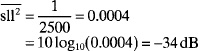
The peak sidelobe level is found by manipulating (3.45).

The peak sidelobe level of this array at which 90% of the sidelobes fall below is given by

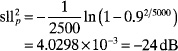
Increasing the probability to 0.99 yields a sidelobe level of

Figure 3.53. The desired Taylor amplitude taper is shown as a solid line. The thinned array amplitude weights are shown as small circles.

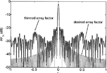
Figure 3.54. The desired array factor (dashed line) is superimposed on the thinned array factor (solid line).

Example. Start with a 100-element array with element spacing d = 0.5λ, and thin to a 20-dB, = 5 Taylor taper.

The normalized amplitude taper shown as a solid line in Figure 3.53 serves as the probability cutoff for selecting elements turned on or off. The small circles at the top or bottom are the amplitude weights of the thinned array. The thinned aperture is not symmetric. The desired and thinned array factors appear in Figure 3.54. The thinned array factor has relatively constant sidelobe levels, while the sidelobes of the Taylor array decrease away from the main beam.

Figure 3.55. Thinned array based upon a 20-dB = 2 Taylor circular amplitude distribution.

Statistical thinning can also be applied to planar arrays [50]. The amplitude taper serves as a two-dimensional proability distribution function. This concepts works for any shape or element spacing.

Example. Statistically thin a circular array with 284 elements and d_x = d_y = 0.5λ to get a 20-dB = 2 Taylor amplitude distribution.
   The resulting thinned aperture is shown in Figure 3.55. Figure 3.56 is the resulting array factor. It has a directivity of 27.2 dB and a peak sidelobe level of 20dB.

The z transform of a thinned linear array is a polynomial with coefficients of either zero or one [51]. As an example, consider a 20-element linear array of isotropic elements. Figure 3.57 is the unit circle representation when the elements are equally weighted and spaced (d = 0.5λ). The nulls in the pattern are equally spaced in phase, Ψ = kdu, but not equally spaced in angle, u. The roots of the uniform array polynomial are given by

Ψ = ±18°, ±36°, ±54°, ±72°, ±90°, ±108°, ±126°, ±144°, ±162°, 180°

If this same array is thinned to obtain the array factor with the minimum maximum sidelobe level, then the second element from each end of the array is turned off (a₂ = 0 and a₁₉ = 0). This configuration yields a far-field pattern that has a maximum sidelobe level of −15.74dB. The unit circle representation and array factor are displayed in Figure 3.58 and Figure 3.59. Note that the zeros are still equally spaced on the unit circle. This pattern appears to have one less zero on the unit circle than the uniform array, because there are double roots at ±60°. The zeros of the thinned array have phases given by

Figure 3.56. Array factor for the thinned array.

Figure 3.57. Unit circle representation of a 20-element uniform array factor with d = 0.5λ.

Ψ = ±20°, ±40°, ±60°, ±60°, ±80°, ±100°, ±120°, ±140°, ±160°, 180°

Since the roots have a magnitude of one, they lie on the unit circle.

Figure 3.58. Unit circle representation of a 20-element array factor when a₂ = 0 and a₁₉ = 0.

Figure 3.59. Array factor of a 20-element uniform array (dotted line) and an array with a₂ = 0 and a₁₉ = 0 (solid line) for d = 0.5λ.

Not all thinned arrays have their roots on the unit circle though. In fact, for the 20-element array, only when one of the element pairs 1 & 20, 2 & 19, 7 & 14, or 10 & 11 are zero will all the roots lie on the unit circle. In all other cases of turning off symmetric pairs of elements, at least one pair of roots will be off the unit circle. Figures 3.60 and 3.61 show an example of the unit circle and far-field pattern of a thinned array with zeros off the unit circle. The array has 20 elements with elements 8 and 13 turned off. The zeros whose magnitudes don’t equal one correspond to the pattern minimum at u = 0.85.

Figure 3.60. Unit circle representation of a 20-element uniform array with a₈ = 0 and a₁₃ = 0.

Figure 3.61. Array factor of a 20-element uniform array with d = 0.5λ having a₈ = 0 and a₁₃ = 0.

3.4.1.2. Thinning Using Numerical Optimization. One way to find the thinned array that results in the lowest sidelobe level is to check every possible array thinning combination. Finding the maximum sidelobe level for 2_N array factors becomes an unreasonable task as N get large. Numerical optimization techniques offer more feasible alternatives to finding the best (or more likely, a very good) solution without resorting to an exhaustive search. Most approaches to numerical optimization require continuous variables and do not adapt well to the on/off condition of thinning. The introduction of genetic algorithms changed the ability to thin arrays [52]. Arrays thinned with genetic algorithms have a higher taper efficiency and lower sidelobe levels than do previous numerical and statistical approaches. Numerical optimization offers several advantages over statistical thinning:

1. The maximum sidelobe level can be specified (as long as it is physically possible).
2. Higher efficiency.
3. Works for small and medium-sized arrays.

The genetic algorithm can also be used to thin planar arrays [53, 54].

Example. Use a genetic algorithm to thin a 50-element linear array with d = 0.5λ to obtain the lowest sidelobe level.

The cost function requires both end elements and both center elements of the array to have an amplitude of one in order to minimize the maximum sidelobe level. The thinned array has η_T = 0.80 and a maximum sidelobe level of −17.6 dB. The array factor is shown in Figure 3.62.

Figure 3.62. This array factor results from using a genetic algorithm to thin a 50-element array.

Figure 3.63. Thinned uniform concentric ring array having 9 rings.

Example. Use a genetic algorithm to thin a uniform concentric ring array with 270 elements layed out in nine rings spaced λ/2 apart and having d_n = 0.5λ to obtain the lowest sidelobe level.

The thinned aperture is shown in Figure 3.63. It only has 66.3% of the 279 elements in the fully populated array. Turning off 94 of the elements reduced the directivity to 27.17 dB and the maximum relative sidelobe level to 22.44 dB. Since the thinning is not symmetric, the array factor is not symmetric either (Figure 3.64). The number of elements in each ring is shown in Table 3.3. The inner five rings have between 0% and 13% of the element removed, while the outer four rings have between 30% and 60% of the elements removed.

3.4.2. Nonuniformly Spaced Arrays

Thinned arrays have a large but finite number of possible active element locations. In contrast, nonuniformly spaced or aperiodic arrays have an infinite number of possible element locations. All elements in nonuniformly spaced arrays are active. Initial attempts at nonuniformly spaced arrays were based upon trial and error. Thinned arrays are more desirable than nonuniformly spaced arrays, because the feed network for the thinned arrays is much easier to design. Also, mutual coupling effects are easier to characterize for periodic array spacing than for aperiodic spacing. Also, implementing nonuniform spacing on planar arrays is extremely difficult.

3.4.2.1. Density Tapering. Density tapering for a nonuniformly spaced linear array differs from density tapering for thinned arrays in that the element spacing is related to the desired amplitude taper rather than the probability of whether an element in an equally spaced array is on or off. The idea is to divide the area under the desired amplitude taper into N equal sub-areas. An element is placed at the point that equally splits each sub-area.

Figure 3.64. Array factor of the thinned uniform concentric ring array.

TABLE 3.3. Ring Radius and Number of Elements per Ring for a Nine-Ring Uniform Thinned Concentric Ring Array

Example. Find the density taper for a 15-element array that mimics a 20-dB, = 3 Taylor taper. Figure 3.65 shows the desired amplitude taper as a dashed line. The dotted vertical lines divide the area under the amplitude taper into 15 equal sub-areas. An element is placed at the point that evenly divides a sub-area (small circles). Figure 3.66 is the resulting array factor due to the nonuniform spacing. The pattern accurately reproduces the desired Taylor pattern out to about u = ±0.5. This technique does not work well for very low sidelobes. Even a 20-dB Taylor taper cannot be accurately reproduced.

3.4.2.2. Fractional z-Transform Synthesis. Earlier in this chapter, the unit circle representation of thinned arrays was introduced. For the more general case of nonuniformly spaced arrays, the far-field pattern is not represented by a polynomial, so polynomial root finding techniques cannot be applied [51]. An approach to adapting the unit circle representation of a nonuniformly spaced array can be found by examining roots of a 4-element array that is symmetric about its center. It has an array factor given by

Figure 3.65. Taylor 20-dB taper is divided into equal areas, and an element is placed at the center of each area.

Figure 3.66. Taylor 20-dB array factor from density tapering.

where s₁ and s₂ are the distances of the center and edge elements from the center of the array. Using a trigonometric identity and substituting = kdu (d = 2s₁) allows the array factor to be written as

This equation is zero when either

Thus, the location of the roots on the unit circle are a function of the spacings and are given by

The zeros of larger arrays are more difficult to find and are not always on the unit circle.

Consider an N element linear array of equally weighted, nonuniformly spaced point sources. Its array factor is represented by

where s_n is the distance of element n from the first element. The phase terms of this equation are not harmonics in a Fourier series. In order to write (3.50) in terms of a z transform, let d_min = minimum spacing between any two adjacent elements [55]. Next find = kd_minu. Equation (3.50) is then written as

Making the substitution yields

Equation (3.52) is a polynomial when s_n/d_min are integers. When z is raised to a noninteger power, this representation is known as a fractional z transform [55]. Only the roots for which |u| ≤ 1 are valid. All others are ignored.

Example. Find the roots on the unit circle corresponding to an array with the element spacings given by

s_n = 0, 1, 1.9, 2.7, 3.4, 4.0, 4.5, 5.0, 5.5, 6.0, 6.5,
    7.0, 7.5, 8.0, 8.5, 9.1, 9.8, 10.6, 11.5, 12.5λ

The array factor with z = e^jk(0.5)μ is written as

This equation can be converted to a polynomial by letting z = e^jk(0.1)μ.

Factoring this polynomial yields 125 roots. Only the roots for |μ| ≤ 1 exist and are given by

μ = ±0.0953, ±0.143, ±0.216, ±0.304, ±0.366, ±0.440, ±0.521,
±0.819, ±0.901, ±0.988                                                      

Plots of the far-field pattern and unit circle representation are shown in Figures 3.67 and 3.68, respectively. Note that there are 26 zeros to (3.54) even though there are only 20 elements. Since the average separation between element is 0.66λ, there are more nulls.

If d is very small, then the maximum power of z can be quite large for even a small array. One way to increase the size of s is to first round or quantize the value of s_n. The value of s will quantize the spacing of the array elements and produce an error in the array factor. This quantization error must produce error sidelobe levels less than the desired sidelobe level of the array.

Figure 3.67. Unit circle representation of the 20-element nonuniformly spaced array.

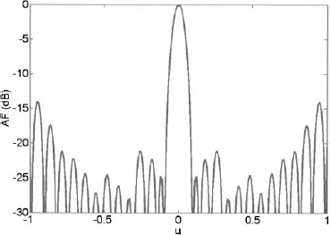
Figure 3.68. Array factor of the 20-element nonuniformly spaced array.

3.4.2.3. Minimum Redundancy Arrays. Large, sparsely populated arrays are used to observe faint extragalactic radio sources, because they have a narrow main beam and are economical (use only a few elements). A minimum redundancy array is a sparse array that maximizes the distance between grating lobes while maintaining the sidelobes in between the grating lobes at a relatively constant level. Its narrow beamwidth scans distant sections of space while keeping the grating lobes out of those sections. The distance between the first grating lobe and the main beam can be maximized while minimizing the number of elements by including all of the integer multiples of the fundamental spatial frequencies only once. The fundamental spatial frequency is given by one over the minimum element spacing

The other spatial frequencies are just multiples (harmonics) of f_s. A 5-element uniform array has N – 1 = 4 representations of f_s, 3 of 2f_s, 2 of 3f_s, and 1 of 4f_s. The highest spatial frequency, f_s, is due to the total aperture length. Higher resolution is possible when the number of redundant spacings are reduced. The number of distinct elements which can be resolved in a linear array is approximately equal to (N – 1)d, and this is obtained when the angular width of the source is equal to the separation between the grating lobes. When the size of the source is known (e.g., the sun), the grating lobe spacing should be matched to the source size. Figure 3.69 shows a 4-element minimum redundancy array and its array factor when d = 1.5λ and the first grating lobe occurs at 48.2°. A completely nonredundant linear array must have less than 5 elements. Looking at the separation distances between all possible combinations of two elements in the array reveals that each integer multiple of d up to the length of the array d, 2d, ..., 6d occurs once and only once. Arrays with more than 4 elements will have more than one sample at some spatial frequencies. The redundancy factor is given by [56]

Figure 3.69. Array factor for a 4-element minimum redundancy array. The array spacing is shown in the upper right corner.

where N is the number of elements in the array and (N_max – 1) × d is the length of the array. Ideally, R should be as close to one as possible (only arrays with less than five elements can have R = 1). The lower limit for R on large arrays is 4/3. Global optimization techniques, such as simulated annealing, are needed to find large minimum redundancy arrays [57].

Example. List the number of possible spatial harmonics associated with a 4-element uniform array, a 7-element uniform array, and a four element minimum redundancy array. Table 3.4 lists the spatial frequencies associated with the arrays. Note that dc refers to a single element.

3.4.2.4. Numerical Optimization of Array Spacing. Finding the element spacings of a uniformly weighted array that produced the lowest possible sidelobe levels was investigated using a genetic algorithm [58]. The cost function is given by

TABLE 3.4. List of Spatial Frequencies in the Arrays

Figure 3.70. Array factor for an optimized element spacing of a 19-element array.

where 2N + 1 is the number of elements, x_n is the location of element n, x₀ = 0, d₀ = λ/2, Δ_n is the variable spacing between 0 and λ/2, and u_MB is the first null next to the main beam. This cost function requires a minimum spacing of d₀, so if all Δ_n = 0, then a uniform array with spacing d₀ results. Since the array is uniformly weighted, the value of u_MB can be approximated by 0.5λ/x_N.

Example. Find the optimum spacing for a 19-element array with d₀ = 0.5λ that yields the lowest sidelobe level.

The genetic algorithm had a population size of 8 and mutation rate of 0.15. After 1000 generations, a Nelder-Mead algorithm polished the results. Figure 3.70 shows the resulting array factor with a maximum sidelobe level of –20.6 dB. The 19 round dots in the figure represent the relative element spacings of the array elements.

3.4.2.5. Nonuniformly Spaced Concentric Ring Array. Nonuniformly spacing the rings in a concentric ring array can also produce low sidelobe levels [54]. First, the rings are assumed to be separated by a minimum distance of λ/2 (not necessary but practical). An additional separation of Δ_n is added to the radius of ring n – 1, so that ring n has a radius of

where 0 ≤ Δ_n ≤ λ. A hybrid genetic algorithm that combines a continuous genetic algorithm with a local optimizer is used to find the r_n that result in the minimum maximum sidelobe level in the array factor. Table 3.5 displays the optimized ring spacing and the number of elements in each ring (keeping d ≃ λ/2). This new array has only 201 elements. The resulting directivity is 27.38 dB and the maximum relative sidelobe level is 22.94 dB. Figure 3.71 is a diagram of the array. The first and last rings have the largest Δ_n. Since the ring separation remains close to λ/2, the sidelobes have sufficient sampling in , and they maintain symmetry in . Figure 3.72 shows the corresponding array factor. All the sidelobes have nearly the same height.

TABLE 3.5. Ring Radius and Number of Elements per Ring for a Six-Ring Nonuniformly Spaced Concentric Ring Array with Optimized r_n

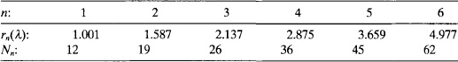
Figure 3.71. Optimized ring spacing for an array with six concentric rings.

Figure 3.72. Array factor associated with optimized ring spacing for an array with six concentric rings.

TABLE 3.6. Ring Radius and Number of Elements per Ring for a Nine-Ring Uniform Concentric Ring Array with Optimized N_n

Another approach to reducing the sidelobe level is to let r_n = nλ/2 and optimize the N_n in order to minimize the maximum sidelobe level. A genetic algorithm is used to find the optimum N_n listed in Table 3.6. The first four rings have the same number of elements as a uniform concentric ring array with λ/2 spacing. The optimized array has 183 elements arranged as shown in Figure 3.73. This array has only 65.6% of the elements of the uniform array. The directivity is 28.5 dB and the maximum sidelobe level is 25.58dB. The array factor shown in Figure 3.74 is nearly circularly symmetric for small θ but not for large θ.

An even more powerful approach is to optimize both the ring spacing and the number of elements in each ring. The maximum radius is slightly less than the maximum radius found by optimizing the r_n alone. Table 3.7 has the ring radii and the number of elements in each ring. This array has 142 elements or 50.9% of the nine-ring uniform concentric array. It has a directivity of 28.89 dB and a maximum relative sidelobe level of 27.82 dB. The optimized array appears in Figure 3.75 with the corresponding array factor in Figure 3.76. All the sidelobes are at nearly the same height.

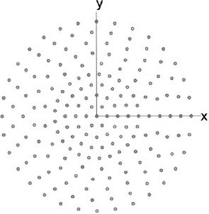
Figure 3.73. Optimized number of elements in nine concentric rings with equal ring spacing.

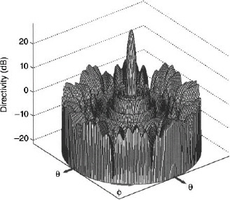
Figure 3.74. Array factor associated with optimized number of elements in nine equally spaced concentric rings.

TABLE 3.7. Ring Radius and Number of Elements per Ring for a Nine-Ring Uniform Concentric Ring Array with Optimized r_n and N_n

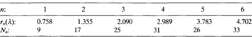
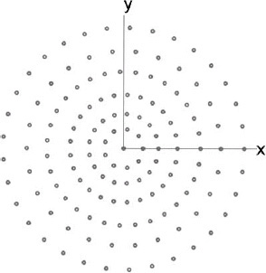
Figure 3.75. Optimized ring spacing and number of elements in each ring for an array with six concentric rings.

Figure 3.76. Array factor associated with optimized ring spacing and number of elements in each ring for array with six concentric rings.

TABLE 3.8. Sidelobe Level Increase as a Result of a 5% Increase in Frequency

Array	Sidelobe Level Increase (dB)
Optimized rn	0.1
Optimized Nn	3.1
Optimized rn and Nn	11.6

The peak sidelobe level of the optimized concentric ring arrays will not change if the frequency decreases by 10%. The sidelobes do not increase because the spatial sampling gets better as the frequency goes down. Increasing the frequency by 5%, however, results in significant sidelobe level increases. Table 3.8 summarizes the sidelobe level increases with a 5% frequency increase. The optimized r_n and N_n case had the greatest increase in sidelobe level, while the optimized ring spacing case has almost no increase. As a result, the array should be optimized at the highest frequency, then the lower frequencies will have low sidelobes.

The concentric ring arrays were optimized without taking scanning into account. When the array beams are scanned, the sidelobe level increases. The nonuniform ring spacing example did not have a sidelobe level increase until the beam was scanned beyond θ = 22.5°. All the other examples experienced increasingly worse sidelobe levels with increasing scan in θ. As an example, steering the main beam in Figure 3.74 to 30° increases the maximum sidelobe level by 8.5 dB. Better performance can be obtained by optimizing over all the scan angles.

3.5 LOW-SIDELOBE PHASE TAPER

A phase taper is another approach to lowering sidelobes in the array factor [59]. The synthesis of a phase taper for an array with uniform amplitude weights and spacing is formulated as a minimization of the maximum sidelobe level [60]. One possible cost function for the numerical optimization of the phase, δ_n, in an N-element array is

where u_mb is the maximum angle of the main beam. The advantage of a phase taper is that low sidelobe levels can be obtained through adjustments to the beam-steering phase shifters rather than by any amplitude weighting via the feed network. These tapers have a modest ability to lower sidelobes and tend to be less efficient than amplitude tapers.

Example. Find a phase taper that results in the lowest possible sidelobe level for a 20-element array with d = 0.5λ.

Figure 3.77. The optimum phase taper for the 20-element array.

Figure 3.78. The array factor due to the phase taper.

A hybrid genetic/Nelder–Meade algorithm was used to find the phase weights. The resulting weights are shown in Figure 3.77 and the associated array factor appears in Figure 3.78. The maximum sidelobe level is 16.1 dB below the peak of the main beam with η_T = 0.84. The resulting phase taper for the right-hand side of the array is

2π (0.145 0.149 0.144 0.153 0.168 0.207 0.231 − 0.0312 0.155 0.101)

For comparison, a 20-element Chebyshev array with a 16.1-dB sidelobe level has η_T = 0.91; and a 16.1-dB, = 2 Taylor array has η_T = 0.98.

3.6 SUPPRESSING GRATING LOBES DUE TO SUBARRAY WEIGHTING

3.6.1. Subarray Tapers

For most applications, placing the weights at the subarray ports alone produces unacceptable grating lobes in the array factor. Minimum sidelobe level in the array factor cannot be less than the highest grating lobe. This is demonstrated in Figure 3.79. The array has 128 elements, 16 subarrays, and an element spacing of 0.5λ. A genetic algorithm optimizes the amplitude weights at the subarray ports while the element weights are uniform. The sidelobe levels next to the main beam are at the same level as the first grating lobe. In order to further reduce the peak sidelobe level, the grating lobes must be dealt with at the element level.

A tradeoff exists between attaining the desired low-sidelobe performance and simplicity of design. One approach places a low-sidelobe amplitude taper at the subarray outputs while the element weights are the same for each subarray [61]. The linear subarray model in Figure 3.80 has amplitude weights at the elements as well as at the subarray ports. All subarrays have identical amplitude tapers across the elements. The elements are assumed to be equally spaced and have symmetric weights about the center of the array. Based upon these assumptions, the array factor for a linear array along the x axis is given by where a_m represents element amplitude weights, b_q represents subarray amplitude weights, 2N_s is the number of subarrays, N_e is the number of elements in a subarray, and θ is the angle from boresight. The effective weights are then represented by a 2N_s × N_e row vector.

Figure 3.79. Array factor for 128-element linear array with 16 subarrays. The amplitude weights at the subarray ports are optimized to give the lowest maximum sidelobe level.

Figure 3.80. Subarrayed antenna with subarray weights and identical element weights in each subarray.

Optimizing the subarray and element weights results in a low-sidelobe array factor with a simplified array design. This approach produces identical corporate feeds for all subarrays and T/R modules weight the signals at the subarray ports.

Example. Find the subarray and element amplitude tapers (same for each subarray) for a 144-element array with (d = 0.5λ) that produces the minimum maximum sidelobe level.

Assume that the array is symmetric about its center. The array has 12 subarrays of 12 elements. Breaking the array into 12 equal-sized subarrays results in 16 optimization variables (11 element amplitude weights and 5 subarray amplitude weights), since a₁ = 1 and b₁ = 1 and the subarray weights are symmetric. A genetic algorithm is used to find the weightings in Figure 3.81 to Figure 3.83. The resulting array factor is shown in Figure 3.84. Grating lobes normally occur in this array at 9.6°, 19.5°, 30.0°, 41.8°, 56.4°, 90.0°. Arrows in Figure 3.84 point to these grating lobe locations. The array directivity is 20.2dB with a peak sidelobe level of −35.9 dB.

The array factor for a planar array in the x−y plane that is symmetric about the x and y axes is given by [62] where a_mn represents element weights, b_pq represents subarray weights, 2N_sx is the number of subarrays in x direction, 2N_sy is the number of subarrays in y direction, N_ex is the number of elements in a subarray in x direction, N_ey is the number of elements in a subarray in x direction, d_x is the element spacing in x direction, and d_y is the element spacing in y direction. A diagram of this array is shown in Figure 3.85. The array is divided into 6 × 6 subarrays each having 5 × 5 elements. A dark color indicates a high-amplitude weight at the element (a_mn). Note that the shade of the dots for each element is the same for every subarray. The tint of the subarray squares is proportional to the subarray weight (b_pq).

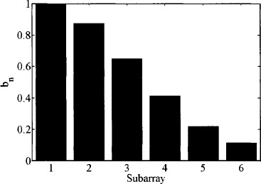
Figure 3.81. Optimized subarray weights when the element weights are identical for all subarrays.

Figure 3.82. Optimized element weights in the subarrays.

Figure 3.83. Effective element weights resulting from the product of the element weight times its corresponding subarray weight.

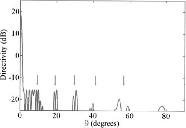
Figure 3.84. Resulting array factor from the optimized weights. Arrows point at the grating lobe locations.

Example. Find the subarray and element amplitude tapers (same for each subarray) for a planar array with with 8 × 8 subarrays each having 8 × 8 elements (d_x = d_y = 0.5λ) that produces the minimum maximum sidelobe level. Assume that the array is symmetric about its center.

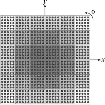
Figure 3.85. Planar array with 6 × 6 subarrays each having 5 × 5 elements. All element weights are the same for all subarays. Darker dots have higher amplitudes than lighter dots. Darker subarrays have higher amplitudes than lighter subarrays.

Since the array is symmetric, there are 15 unknown subarray weights and 63 unknown element weights for a total of 78 unknown variables. A genetic algorithm is used to find these variables. The optimized subarray weights appear in Figure 3.86 with the optimized element weights in Figure 3.87. Figure 3.88 shows the product of the element weights times the subarray weights. The resulting array factor is shown in Figure 3.89. This array factor has a directivity of 34.7 dB with a maximum relative sidelobe level of 23.6 dB.

3.6.2 Thinned Subarrays

Figure 3.90 is a diagram of a 256-element square array divided into 16, 4 × 4 element thinned subarrays [63]. Dark circles indicate that the element has an amplitude of one, and white circles indicate that the element is terminated in a matched load and receives an amplitude of zero. Note that the subarrays are either identical or are mirror images.

A genetic algorithm is used to simultaneously optimize the subarray amplitude weights and the thinning for the subarrays. The cost is the maximum relative sidelobe level and is calculated from the array factor given by where w_n is the product of element weight and subarray weight for element n, and (x_n, y_n) is the location of element n.

Figure 3.86. Optimized subarray weights for one quandrant when the element weights are identical for all subarrays.

Figure 3.87. Optimized element weights in the subarrays.

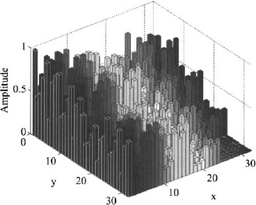
Figure 3.88. Effective element weights resulting from the product of the element weight times its corresponding subarray weight.

Figure 3.89. Resulting array factor from the optimized weights.

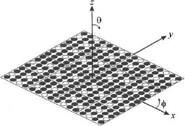
Figure 3.90. Planar array with identically thinned subarrays.

Example. An array has 6 × 6 = 36 subarrays with each subarray having 5 × 5 = 25 elements. The element spacing in both directions of the square lattice is one-half wavelength. Find the thinned subarrays and subarray weights that minimize the maximum sidelobe level.

When the element thinning and subarray weights are simultaneously optimized, then the optimized element weights are shown in Figure 3.91 and the optimized subarray weights are shown in Figure 3.92. When multiplied together, the effective element weights for one quadrant of the array are shown in Figure 3.93. This taper has an efficiency of 54.5%. The resulting array factor appears in Figure 3.94. Its directivity is 26.9 dB and the maximum sidelobe level is −22.9 dB. Sidelobes that are 4.5 dB lower than the optimized subarray weighting come at a cost in taper efficiency and loss in directivity.

One way to eliminate the grating lobes is to create overlapped subarrays. Although difficult to do with corporate array feeds, they can be realized using a Butler matrix or lens feeds that will be discussed in a later chapter. Some examples of implementing a partially overlapped constrained feed network are found in references 64 and 65. Several approaches to amplitude weighting the subarray outputs of identical subarrays exist. Other approaches have tried randomizing the number of elements within a given subarray [66], rotating the subarray orientation [67], and nonuniformly spacing the elements within the subarrays [68, 69]. These methods are designed to break the periodicity and redistribute the energy in the grating lobes throughout the far-field pattern.

Figure 3.91. Optimized subarray weights for one quadrant of the array.

Figure 3.92. Optimized element weights in one subarray.

Figure 3.93. Optimized effective element weights in one quadrant of the array.

Figure 3.94. Optimized array factor.

If an array has subarrays of different sizes and has amplitude weights at the subarray ports when all element weights are one (Figure 3.95), then the effective element weights are given by [70]

Figure 3.95. Diagram of an antenna with unequal sized subarrays and amplitude weights at the subarray ports.

N_e is a vector that is N_s (number of subarrays) long. The total number of elements in the array is given by

A genetic algorithm chromosome or input vector to the cost function consists of 2 × (N_s − 1) values

Since b₁ = 1 and N_e(N_s) = N_T − . The minimum number of elements that are allowed in a subarray is represented by N_emin. Each subarray starts by having N_emin elements. The remaining N_T − N_s × N_emin elements are distributed among the subarrays. Although not necessary, the array is assumed to have an even number of subarrays, and the subarrays are symmetric about the center of the array. Selecting N_emin is arbitrary unless certain design constraints exist. A design constraint may have to do with the way the elements are fed via a corporate feed. For example, all subarrays may have the number of elements equal to a power of two. N_emin has to be at least greater than or equal to two, otherwise the subarrays consist of only a single element. In order to take advantage of the efficiencies offered by subarrays, it will be assumed that the minimum number of elements in a subarray is greater than or equal to four.

Example. Assume a symmetric array (d = 0.5λ) has N_T = 128 elements with N_emin = 4 and N_s = 16. Optimize the subarray weights and sizes to get the minimum maximum sidelobe level.

Figure 3.96. Effective element weights when the subarray weights and number of elements in the subarray are optimized for N_emin = 4 and N_s, = 16.

Figure 3.97. Array factor associated with the weights in Figure 3.96.

A genetic algorithm is used to find the weights and sizes shown in Figure 3.96. The resulting array factor is shown in Figure 3.97. The maximum sidelobe level is 35.9 dB below the peak of the main beam, and the directivity is 19.89 dB.

Figure 3.98. Effective element weights when the subarray weights and number of elements in the subarray are optimized for N_emin = 6 and N_s = 16.

Figure 3.99. Array factor associated with the weights in Figure 3.98.

Example. Assume a symmetric array (d = 0.5λ) has N_T = 128 elements with N_emin = 6 and N_s = 16. Optimize the subarray weights and sizes to get the minimum maximum sidelobe level.

A genetic algorithm is used to find the weights and sizes shown in Figure 3.98. The resulting array factor is shown in Figure 3.99. The maximum sidelobe level is 35.1 dB below the peak of the main beam, and the directivity is 19.93 dB.

Figure 3.100. Array factor associated with the weights in Figure 3.98.

Another way to lower sidelobe levels with uniformly weighted elements (a_n = 1) and subarrays (b_n = 1) breaks the array into N_s subarrays that are symmetric about the center of the array. Subarray n has N_n elements with an element spacing of d_n as shown in Figure 3.100. This approach has been shown to be useful for linear and planar arrays [71].

Example. Assume that a linear array has 64 elements and is divided into three subarrays. Also, d₃ > d₂ > d₁ > 0.5λ and a subarray must have at least one element.

A genetic algorithm found the following array variables:

d₁ = 0.501 λ, d₂ = 0.906λ, d₃ = 1.890λ and N₁ = 21, N₁ = 9, N₁ = 2

The resulting array factor in Figure 3.101 has a directivity of 18.05 dB and a −22.4-dB maximum sidelobe level.

Optimizing a phase taper on an array with a low-sidelobe amplitude taper at the subarray ports (b_n) and uniform amplitude taper at the elements reduces the grating lobe levels (a_n = 1) [72].

Example. Find the element phase taper that best approximates a Taylor distribution with SLL = −30 dB and = 4. The array has 128 elements spaced λ/2 apart and has 8 subarrays with 16 elements per subarray.

The array is optimized using the iterative projection method (IPM) [73] in order to closely approximate the Taylor taper. By exploiting the efficiency in computing discrete Fourier transformations, the IPM is based on an iterative algorithm where the array illumination function is projected onto the corresponding space of far field patterns and then vice versa, until a desired pattern is synthesized. The amplitude taper appears in Figure 3.102 and the optimized phase taper in Figure 3.103. Figure 3.104 shows the peak sidelobe level is reduces by nearly 4 dB. The array without the phase taper has a directivity of 20.3dB and a 3-dB beamwidth of 1.01°, while with the phase taper it has a directivity of 20.1 dB and a 3-dB beamwidth of 1.05°.

Figure 3.101. Array factor for the optimized subarray spacings.

Figure 3.102. Element amplitude weights.

3.7. PLANE WAVE PROJECTION

Measuring far-field antenna patterns requires separating the transmit antenna and the antenna under test (AUT) by a large distance in order to minimize the amplitude and phase variations across the test aperture. When the AUT is many wavelengths across, the far-field distance can become quite large (recall IEEE definition of far field from Chapter 1). Thus, in order to measure the antenna pattern of an electrically large aperture indoors, techniques like compact ranges, near-field scanning, and antenna focusing are necessary. These approaches allow for accurate prediction of the far field pattern even though the measurements are taken in the near field.

Figure 3.103. Element phase weights.

Figure 3.104. Array factors with and without element phase tapers.

A number of techniques have been developed to project a plane wave in the near field of an array by synthesizing appropriate complex element weights. Hill used a constrained least squares approach developed to find the weights that approximate a plane wave in the near field [74]. The results show a flat amplitude response for small linear arrays of line sources. Unfortunately, the phase response, which determines the far field criterion, is not shown. This approach was experimentally applied to a seven element array of Yagi-Uda antennas at 500 MHz [75], In another study, a ring array was synthesized to create a plane wave inside the ring [76], For further background information on creating a plane wave in the near field, the reader is referred to reference 77. A more recent method was developed to create a plane wave in the near field from a linear array of line sources [78] using a genetic algorithm. This approach combines the ideas of array focusing and a compact range. The location and weights of an array of line sources were found that approximate a plane wave at a desired location in space. The optimized amplitude and phase ripples across the AUT are much less than those created by a uniform array with the same number of elements. The resulting plane wave is robust in bandwidth and physical depth. This method also proved successful in experimental testing as reported in references 79 and 80. The idea behind these papers is to find the amplitude, phase, and position of the elements that create a relatively constant field amplitude and phase over a desired area in the near field. A linear array can only control the field in the plane of the array but not the field in the orthogonal plane.

A linear system of equations based on the near field array factor of the array is given by

Figure 3.105 is a diagram of the plane wave projection layout. When M = N, then a direct solution to (3.67) is possible. Otherwise, when M > N (more field points than elements), a least squares solution is found. Since the exact field values at the plane wave is unknown, the amplitude is assumed to be one and the phase zero. Once the weights are found, then they are normalized.

Solving (3.67) yields weights that produce a very flat amplitude and phase field distribution over the plane wave region. In fact, using M = 81 sample points in the first quadrant (Figure 3.105) results in weights that produce a maximum amplitude variation across the plane wave region of 0.003 dB and a phase variation of 0.02°. These amazing results are at a cost, however. Unfortunately, the very flat amplitude response in the desired plane wave region, but the level is at about −70 dB compared to the +5 dB for a uniform array. The amplitude of this plane wave would be in the noise level of an experimental setup, making this approach impractical.

The plane wave appears at such a low level because half the array weights are out of phase with the other half; in other words, it is a difference pattern with a null in the main beam. In the far field, the 1/R_mn terms are replaced by a constant 1/R that can be factored out of the summation. In addition, symmetry can be imposed on both the amplitude and phase of the array weights in the form of combining symmetric phase terms using Euler’s identity for cosine. In the near field, however, R_mn is not a constant and the amplitude of symmetric phase terms are not the same, so symmetry cannot be imposed. Consequently, numerical optimization must be used to find an acceptable solution.

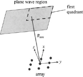
Figure 3.105. Plane wave projection.

The least squares constraint requires that

where C is a constant. Unfortunately, the Green’s function matrix has a large condition number (on the order of 10¹⁰), so when the Hermitan matrix is formed from the Green’s function matrix, the condition number is even higher (on the order of 10¹⁷). This condition number invalidates any results obtained with double precision arithmetic. Thus, another approach is needed for this planar array configuration.

Consider a 6 × 6 element transmitting array with elements arranged in a square lattice with spacings d_x = 1.0λ and d_y = 1.0λ. These large spacings reduce mutual coupling effects, making the point source model a better approximation to reality. Optimized spacings [81] were on the order of a wavelength or larger. The desired 4λ × 4λ plane wave region is z₀ = 10λ away from the transmitting array. This distance is much less than the far field at R_ff = 64λ. Moving this plane wave region to R_ff = 64λ would result in a phase variation of 22.5° and amplitude variation of 0.33 dB. The plane wave region at z₀ = 10λ has a maximum phase deviation of 60° and a maximum amplitude variation of 8.6 dB. These variations exceed the IEEE standard and are unacceptable for most measurements.

The cost function used for the genetic algorithm optimization of the plane wave generator is given by

where E_m are the complex field samples from the desired plane wave region. The first term in the cost function is the maximum phase deviation normalized to π. As long as the plane wave area is not too large, this term stays less than one. The second term is the normalized maximum field amplitude. These terms can be weighted to achieve a desired emphasis on either the field amplitude or phase. In this example, they are weighted equally.

The continuous parameter genetic algorithm used a population size of 80 with 1% mutation rate, 50% crossover rate, and single-point crossover. The amplitude and phase weights for the elements in one quadrant of the array are shown in Table 3.9. The maximum field amplitude variation across the desired plane wave region is 0.75 dB as seen in the contour plot of Figure 3.106. The maximum field phase variation across the desired plane wave region is 32.4° as seen in the contour plot of Figure 3.107. These field variations are a significant improvement over the same field variations due to a uniform array.

3.8 INTERLEAVED ARRAYS

Placing multiple antennas in the same area is important when space is limited as on a satellite. Antenna arrays that occupy the same area are called shared or common apertures. In these arrays, groups of elements dedicated to different frequencies or functions are interleaved, interlaced, or interspersed within the same aperture.

Interleaving elements dedicated to different feed networks have been successful in many applications. Random interleaving of elements in adjacent subarrays disrupt the grating lobes that result when only one phase shifter per subarray is used to steer the beam. Randomly assigning elements to subarrays reduces the peak sidelobe level. Interleaved arrays of waveguide radiators operating at different frequencies have been built [82], An aperture with three arrays of interleaved elements operating in the L, S, and C bands was successfully built and measured to demonstrate the feasibility of interleaving three arrays on the same aperture [83]. A dual-band phased array using interleaved waveguides (C band) and printed dipoles on a high dielectric substrate (S band) has been developed. The element spacings for both arrays were equal, so no grating lobes formed in either band [84], A phased array antenna with interleaved waveguide elements and wideband tapered elements was shown to operate over at least three frequency bands [85]. A dual-band/dual-polarization array had an interleaved cross-dipole radiator and a cavity-backed disk radiator in the same lattice structure [86], Most interleaved arrays consist of multiple arrays operating at different frequencies.

TABLE 3.9. The Optimized Weights Found by the Genetic Algorithm

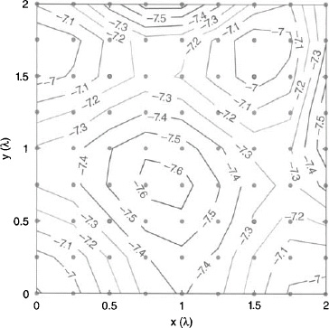
Figure 3.106. Field amplitude distribution (in decibels) at the plane wave area.

Figure 3.107. Field phase distribution in degrees at the plane wave area.

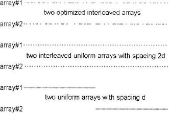
Figure 3.108. Two arrays occupying the same aperture size. The bottom arrays are two 30-element uniformly spaced arrays placed side by side (d = 0.5λ). The center two arrays have every other element turned on resulting in two arrays with d = 0.5λ. The top two arrays were optimized to create the lowest maximum sidelobe.

There are several ways to have two arrays operating at the same frequency share the same aperture. Placing one array on the left side of the area and the other array on the right side of the area does not make use of any interleaving (bottom of Figure 3.108). The array factor of these arrays with N = 30 is shown in Figure 3.109 for d = 0.5λ. Another approach interleaves the two arrays with every other element feeding one array and the remaining elements feeding the second array. The pattern of one of the arrays having d = 1.0λ is in Figure 3.109. The side-by-side arrays have the advantage of lower average sidelobe levels while the every other element interleaved arrays have the advantage of narrower beamwidth. Each array in the aperture has η_t = 0.50, but the whole aperture has η_t = 1.00.

A genetic algorithm can optimize the interleaving of two antisymmetrically thinned arrays to minimize the maximum sidelobe level [87]. When one array has an element on/off, the other array has it off/on, so the amplitude weights for the first array are represented as

and those for the second array are expressed as

The genetic algorithm found the optimum thinning configuration for a 60-element array shown at the top of Figure 3.108, and the pattern of one of these arrays is the solid line in Figure 3.109. Adding w to w′ yields a vector of all ones which implies η_ap = 100% with each array having η_ar = 50%. The symmetry associated with w and w′ ensures that 50% of the elements will be turned on in each array. The arrays have nearly the narrow beamwidth of the full aperture and has the same peak sidelobe level of a uniform array. The resulting arrays are a compromise between the side-by-side uniform array and the every-other element interleaved array.

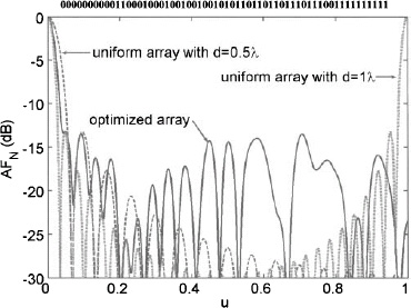
Figure 3.109. Array factor for an optimized fully interleaved array is compared to the array factors for a side-by-side array (d = 0.5λ) and every other element interleaved array (d = 1.0λ) when there are 60 total elements with 30 turned on.

Example. Find the interleaved configuration that yields the lowest maximum sidelobe level for two 10-element arrays with d = 0.5λ.

A genetic algorithm optimized the interleaved arrays to get the following weights:

w = [11111111101000000000]

The maximum sidelobe level of the optimized array factor in Figure 3.110 is −14 dB.

A thinned sum array has the highest density of elements turned on in the center corresponding to the desired low sidelobe amplitude tapers. A low-sidelobe thinned difference array has few elements turned on in the center. Both arrays have less “on” elements near the edges. Using the elements turned “off” in an optimally thinned sum array to create a thinned difference array does not result in an acceptable difference pattern [87].

Figure 3.110. Array factor associated with two 10-element interleaved arrays.

Figure 3.111. Sum array factor due to interleaved thinned sum and difference arrays.

If the thinned difference array has elements turned off then the sum array or b_n = 1 − a_n. A genetic algorithm found the thinning arrangement that results in the minimum maximum sidelobe level for both array factors results in an array having the patterns shown in Figure 3.111 and Figure 3.112. The patterns are normalized to their respective peaks. The peak sidelobe level of the sum pattern is 12.68 dB below its main beam, and the peak sidelobe level of the difference pattern is 12.5 dB below its main beam. The sum array has η_ar = 0.48 and the difference array has η_ar = 0.52. The entire aperture is 100% efficient, so optimum use is made of the available space.

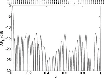
Figure 3.112. Difference array factor due to interleaved thinned sum and difference arrays.

3.9. NULL SYNTHESIS

Earlier in this chapter, the z transform was used to move nulls to get low sidelobes and place nulls in the array factor at desired angles. That approach does not take into account the distortion to the array factor caused by the null placement. In this section, the null placement is done with minimal distortion to the array factor [88].

Element weights can be found that place nulls at M locations in the array factor. Assume that the new weights are given by

where a_n is the amplitude taper and Δ_n is the complex weight perturbation that causes the nulls. Substituting (3.72) into the equation for a linear array factor results in a nulled array factor that is the sum of the quiescent array factor and a cancellation array factor.

There are an infinite number of combinations of w_n that result in nulls in the M desired directions. Writing (3.73) in matrix form results in

where

Since (3.74) has more columns than rows, finding the weights requires a least squares solution in the form [89]

Example. A 40-element array of isotropic point sources spaced λ/2 apart has a 30-dB, = 7 Taylor taper. Plot the array factors and cancellation beam for a null at 61°. The adapted array factor is very close to the quiescent pattern (Figure 3.113), except near the nulls. Note that the cancellation pattern equals the height of the quiescent patterns where the nulls occur. The cancellation beam has the same Taylor taper as the quiescent pattern. The low sidelobes of the cancellation beam ensures that the pattern away from the null is minimally perturbed.

Example. Repeat the last example for nulls at 13° and 61°.

Figure 3.114 shows that both nulls are placed with little perturbation to the pattern except for the sidelobes on either side of the nulls.

Ideally, the quiescent pattern should be perturbed as little as possible when placing the nulls. The weights that produce the nulls are [90]

where γ_m is the sidelobe level of the quiescent pattern at u_m and c_n is the amplitude taper of the cancellation beam. When c_n = a_n, the cancellation pattern looks the same as the quiescent pattern. When c_n = 1.0, the cancellation pattern is a uniform array factor and is the constrained least mean square approximation to the quiescent pattern over one period of the pattern. The nulled array factor can now be written as Equation (3.77) works because the cancellation beams are orthogonal: When cancellation pattern m has a peak at u_m, all the other cancellation patterns have nulls.

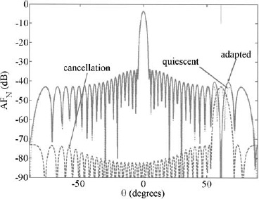
Figure 3.113. Adapted array factor with quiescent and cancellation pattern for a null at 61°.

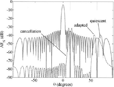
Figure 3.114. Adapted array factor with quiescent and cancellation pattern for nulls at 13° and 61°.

Figure 3.115. Adapted array factor with quiescent and weighted cancellation patterns for nulls at 13° and 61°.

Example. Repeat the previous example using both uniform and weighted cancellation beams.

The weighted cancellation beam (Figure 3.115) causes the sidelobes to become higher on either side of the null more than the uniform cancellation beam, because the uniform cancellation beam has a narrower beamwidth. The uniform cancellation beam (Figure 3.116) raises the sidelobe level in other places more than the weighted cancellation beam, because it has higher sidelobe levels (look at ±90°).

This procedure extends to phase-only nulling. When the phase shifts are small, then e^jn ≈ 1 + j_n, and the array factor can be written as [91]

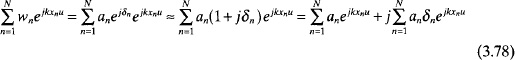
Using Euler’s identity, (3.78) is written as

Figure 3.116. Adapted array factor with quiescent and uniform cancellation patterns for nulls at 13° and 61°.

Equating the real and imaginary parts of (3.79) leads to

Now, (3.80) is in the form that can be solved via (3.75).

Example. A 40-element array of isotropic point sources spaced λ/2 apart has a 40-dB, = 7 Taylor taper. Plot the array factors and cancellation beams for nulls at 13° and 61°. Use phase-only nulling.

Figure 3.117 is a plot of the quiescent, nulled, and cancellation patterns. Phase-only nulling with minimal weight perturbations results in cancellation beams with peaks at symmetric locations about the main beam [92]. A null is placed in the pattern at the desired location, while the pattern increases at the symmetric location. Note the higher sidelobes at –13° and –61°. Consequently, this approach cannot place nulls in symmetric locations in the array pattern. Larger phase shifts that cause greater pattern distortion are required to place symmetric nulls in the array patterns [93].

Figure 3.117. Adapted array factor with quiescent and uniform cancellation patterns for nulls at 13° and 61°.

A monopulse phased array has separate sum and difference channels. If each channel has a low-sidelobe taper as shown in Figure 3.118, then the shared phase shifters (and amplitude weights) can be used to simultaneously place nulls in the sum and difference patterns. The matrixes in (3.74) are now written as [94]

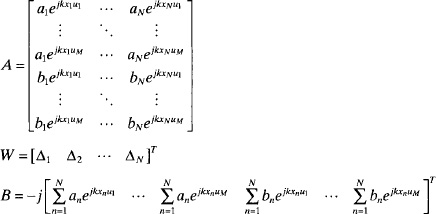
Phase-only nulling requires further simplification as noted in (3.79).

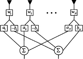
Figure 3.118. Diagram of an array with low-sidelobe sum and difference channels.

Figure 3.119. Sum pattern quiescent, nulled, and cancellation patterns for simultaneous nulling in the sum and difference patterns.

Example. A 40-element array of isotropic point sources spaced λ/2 apart has a 30-dB, = 7 Taylor taper and a 30-dB, = 7 Bayliss taper. Plot the array factors and cancellation beams for nulls at 13° and 61°. Use simultaneous phase-only nulling in the sum and difference patterns.

Figures 3.119 and 3.120 are the resulting patterns with deep nulls in the desired directions.

Figure 3.120. Difference pattern quiescent, nulled, and cancellation patterns for simultaneous nulling in the sum and difference patterns.

REFERENCES

1. P. M. Woodward, A method for calculating the field over a plane aperture required to produce a given polar diagram, J. IEE, Vol. 93, Pt. IIIA, No. 37, September 1946, pp. 1554–1558.
2. P. M. Woodward and J. D. Lawson, The theoretical precision with which an arbitrary radiation pattern may be obtained from a source of finite size, J. IEE, Vol. 95, Pt. III, No. 37, September 1948, pp. 363–370.
3. R. L. Haupt and D. H. Werner, Genetic Algorithms in Electromagnetics, New York: John Wiley & Sons, 2007.
4. R. L. Haupt, Genetic algorithm applications for phased arrays, ACES J., Vol. 21, No. 3, November 2006, pp. 325–336.
5. J. S. Stone, US Patent 1,643,323, September 27,1927.
6. C. L. Dolph, A current distribution for broadside arrays which optimizes the relationship between beam width and sidel-lobe level, Proc. IRE, Vol. 34, No. 6, June 1946, pp. 335–348.
7. R. S. Elliott, The theory of antenna arrays, in Microwave Scanning Antennas, R. C. Hansen, ed., New York: Academic Press, 1964, pp. 1–69.
8. F. I. Tseng and D. K. Cheng, Optimum scannable planar arrays with an invariant sidelobe level, IEEE AP-S Trans., Vol. 56, No. 11, November 1968, pp. 1771–1778.
9. Y. V. Baklanov, Chebyshev distribution of currents for a plane array of radiators, Radio Eng. Electron. Phys., Vol. 11,1966, pp. 640–642.
10. T. T Taylor, Design of line source antennas for narrow beamwidth and low side lobes, IRE AP Trans., Vol. 3,1955, pp. 16–28.
11. T. T. Taylor, One parameter family of line sources producing modified symmetry patterns, Report No. TM 324, Culver City, CA: Hughes Aircraft Co., 1953.
12. T. Taylor, Design of circular apertures for narrow beamwidth and low sidelobes, IEEE AP-S Trans., Vol. 8, No. 1, January 1960, pp. 17–22.
13. R. C. Hansen, A one-parameter circular aperture distribution with narrow beam-width and low sidelobes, Vol. 24, No. 4, July 1976, pp. 477–80.
14. W. D. White, Circular aperture distribution functions, IEEE AP-S Trans., Vol. 25, No. 5, September 1977, pp. 714–716.
15. E. T. Bayliss, Design of monopulse antenna difference patterns with low sidelobes, The Bell System Tech. J., Vol. 47, May–June 1968, pp. 623–650.
16. R. S. Elliott, Design of line source antennas for narrow beamwidth and asymmetric low sidelobes, IEEE AP-S Trans., Vol. 23, No. 1, January 1975, pp. 100–107.
17. R. S. Elliott, Antenna Theory and Design, revised edition, Hoboken, NJ: John Wiley & Sons, 2003.
18. C. McCormack and R. Haupt, Antenna pattern synthesis using partially tapered arrays, IEEE Trans. Magn., Vol. 27, No. 5,1991, pp. 3902–3904.
19. W. H. Press et al., Numerical Recipes in FORTRAN, New York: Cambridge University Press, 1992.
20. J. A. Nelder and R. Mead, Comput. J., Vol. 7, 1965, pp. 308–313.
21. D. G. Luenberger, Linear and Nonlinear Programming, Reading, MA: Addison-Wesley, 1984.
22. M. J. D. Powell, An efficient way for finding the minimum of a function of several variables without calculating derivatives, Comput. J., 1964, pp. 155–162.
23. G. C. Broyden, A class of methods for solving nonlinear simultaneous equations, Math. Comput., October 1965, pp. 577–593.
24. R. Fletcher, Generalized inverses for nonlinear equations and optimization, in Nurnerical Methods for Nonlinear Algebraic Equations, R. Rabinowitz, ed., London: Gordon and Breach, 1970, pp. 75–85.
25. D. Goldfarb and B. Lapidus, Conjugate gradient method for nonlinear programming problems with linear constraints, I&EC Fundamentals, February 1968, pp. 142–151.
26. D. F. Shanno, An accelerated gradient projection method for linearly constrained nonlinear estimation, SIAM J. Appl. Math., March 1970, pp. 322–334.
27. M. I. Skolnik, G. Nemhauser, and J. W. Sherman, III Dynamic programming applied to unequally spaced arrays, IEEE AP-S Trans., Vol. 12, January 1964, pp. 35–43.
28. N. Balakrishnan, P. K. Murthy, and S. Ramakrishna, Synthesis of antenna arrays with spatial and excitation constraints, IEEE AP-S Trans., Vol. 27, No. 5, September 1979, pp. 690–696.
29. J. Perini, Note on antenna pattern synthesis using numerical iterative methods, IEEE AP-S Trans., Vol. 12, July 1976, pp. 791–792.
30. C. S. Ruf, Numerical annealing of low-redundancy linear arrays, IEEE Trans., Vol. 41, No. 1, January 1993, pp. 85–90.
31. W. L. Stutzman and E. L. Coffey, Radiation pattern synthesis of planar antennas using the iterative sampling method, IEEE Trans., Vol. AP-23, No. 6, November 1975, pp. 764–769.
32. H. J. Orchard, R. S. Elliot, and G. J. Stern, Optimizing the synthesis of shaped beam antenna patterns, IEE Proc, Vol. 132, No. 1, February 1985, pp. 63–68.
33. R. S. Elliot and G. J. Stearn, Shaped patterns from a continuous planar aperture distribution, IEEE Proc., Vol. 135, No. 6, December 1988, pp. 366–370.
34. J. E. Richie and H. N. Kritikos, Linear program synthesis for direct broadcast satellite phased arrays, IEEE AP-S Trans., Vol. 36, No. 3, March 1988, pp. 345–348.
35. F. Ares, R. S. Elliott, and E. Moreno, Design of planar arrays to obtain efficient footprint patterns with an arbitrary footprint boundary, IEEE AP-S Trans., Vol. 42, No. 11, November 1994, pp. 1509–1514.
36. O. Einarsson, Optimization of planar arrays, IEEE AP-S Trans., Vol. AP-27, No. 1, January 1979, pp. 86–92.
37. T. S. Ng, J. Yoo Chong Cheah, and F. J. Paoloni, Optimization with controlled null placement in antenna array pattern synthesis, IEEE Trans., Vol. AP-33, No. 2, February 1985, pp. 215–217.
38. D. K. Cheng, Optimization techniques for antenna arrays, Proc. IEEE, Vol. 59, No. 12, December 1971, pp. 1664–1674.
39. J. F. DeFord and O. P. Gandhi, Phase-only synthesis of minimum peak sidelobe patterns for linear and planar arrays, IEEE AP-S Trans., Vol. 36, No. 2, February 1988, pp. 191–201.
40. R. L. Haupt, Genetic algorithm applications for phased arrays, ACES J., Vol. 21, No. 3, November 2006, pp. 325–336.
41. S. Kirkpatrick, C. D. Gelatt, and M. P. Vecchi, Optimization by simulated annealing, Science, Vol. 220, No. 4598, May 13,1983, pp. 671–680.
42. N. Metropolis, A. Rosenbluth, and M. Rosenbluth, J. Chem. Phys., Vol. 21, 1953, pp. 1087–1092.
43. J. H. Holland, 1975, Adaptation in Natural and Artificial Systems, Ann Arbor: The University of Michigan Press.
44. D. E. Goldberg, 1989, Genetic Algorithms in Search, Optimization, and Machine Learning, New York: Addison-Wesley.
45. R. L. Haupt and S. E. Haupt, Practical Genetic Algorithms, 2nd edition, New York: John Wiley & Sons, 2004.
46. R. L. Haupt and D. Werner, Genetic Algorithms in Electromagnetics, New York: John Wiley & Sons, 2007.
47. R. Willey, Space tapering of linear and planar arrays, IEEE AP-S Trans., Vol. 10, 1962, pp. 369–377.
48. M. Skolnik, J. Sherman III, and F. Ogg, Jr., Statistically designed density-tapered arrays, IEEE AP-S Trans., Vol. 12, No. 4,1964, pp. 408–417.
49. E. Brookner, Antenna array fundamentals—part 1, in Practical Phased Array Antenna Systems, E. Brookner, ed., Norwood, MA: Artech House, 1991, pp. 2-1–2-37.
50. T. A. Milligan, Space-tapered circular (ring) array, IEEE AP Mag., Vol. 46, No. 3, June 2004, pp. 70–73.
51. R. L. Haupt, Unit circle representation of aperiodic arrays, IEEE AP-S Trans., Vol. 43, No. 9, October 1995, pp. 1152–1155.
52. R. L. Haupt, Thinned arrays using genetic algorithms, IEEE AP-S Trans., Vol. 42, No. 7, July 1994, pp. 993–999.
53. R. L. Haupt, Thinned arrays using genetic algorithms, in Electromagnetic Optimization by Genetic Algorithms, Y. Rahmat-Samii and E. Michielssen, eds., New York: John Wiley & Sons, 1999, pp. 95–117.
54. R. L. Haupt, Optimized element spacing for low sidelobe concentric ring arrays, IEEE AP-S Trans., Vol. 56, No. 1, January 2008, pp. 266–268.
55. V. Namias, The fractional order Fourier transform and its application to quantum mechanics, J. Inst. Appl. Math., 25,1980, pp. 241–265.
56. A. T. Moffet, Minimum-redundancy linear arrays, IEEE AP-S Trans., Vol. 16, No. 2, March 1968, pp. 172–175.
57. C. S. Ruf, Numerical annealing of low-redundancy linear arrays, IEEE AP-S Trans., Vol. 41, No. 1, January 1993, pp. 85–90.
58. R. L. Haupt, An introduction to genetic algorithms for electromagnetics, IEEE Antennas Propagat. Mag., Vol. 37, No. 2, April 95, pp. 7–15.
59. J. F. DeFord and O. P. Gandhi, Phase-only synthesis of minimum peak sidelobe patterns for linear and planar arrays, IEEE Trans. Antennas Propagat., Vol. 36, No. 2, February 1988, pp. 191–201.
60. R. L. Haupt, Optimum quantized low sidelobe phase tapers for arrays, IEE Electron. Lett., Vol. 31, No. 14, July 95, pp. 1117–1118.
61. R. Haupt, Reducing grating lobes due to subarray amplitude tapering, IEEE AP-S Trans., Vol. 33, No. 8, August 1985, pp. 846–850.
62. R. Haupt, Optimization of subarray amplitude tapers, IEEE AP-S Symp., June 1995, pp. 1830–1833.
63. R. L. Haupt, Low sidelobes from identically thinned subarrays, in IEEE AP-S Symposium, Albuquerque, NM, 2006, pp. 4217–4220.
64. R. J. Mailloux, Constrained feed technique for subarrays of large phased arrays, IEE Electron. Lett., Vol. 34, November 12,1998, pp. 2191–2193.
65. R. J. Mailloux, A low-sidelobe partially overlapped constrained feed network for time-delayed subarrays, IEEE AP-S Trans., Vol. 49, February 2001, pp. 280–291.
66. A. P. Goffer, M. Kam, and P. R. Herczfeld, Design of phased arrays in terms of random subarrays, IEEE AP-S Trans., Vol. 42, June 1994, pp. 820–826.
67. P. S. Hall and M. S. Smith, Sequentially rotated arrays with reduced sidelobe levels, IEE Proc. Microwave Antennas Propagat., Vol. 141, August 1994, pp. 321–325.
68. N. Toyama, Aperiodic array consisting of subarrays for use in small mobile earth stations, IEEE AP-S Trans., Vol. 53, June 2005, pp. 2004–2010.
69. K. C. Kerby and J. T. Bernhard, Wideband periodic array of random subarrays, IEEE AP-S Symp., June 2004, pp. 555–558.
70. R. L. Haupt, Optimized weighting of uniform subarrays of unequal sizes, IEEE AP-S Trans., Vol. 56, No. 1, January 2008, pp. 1207–1210.
71. M. Alvarez-Folgueiras, J. Rodriguez-Gonzalez, and F. Ares-Pena, High-performance uniformly excited linear and planar arrays based on linear semiarrays composed of subarrays with different uniform spacings, IEEE AP-S Trans., Vol. 57, December 2009, pp. 4002–4006.
72. P. Rocca, R. L. Haupt, and A. Massa, Sidelobe reduction through element phase control in uniform subarrayed array antennas, IEEE AWPL, Vol. 8, 2009, pp. 437–440.
73. O. M. Bucci, G. Franceschetti, G. Mazzarella, and G. Panariello, Intersection approach to array pattern synthesis, Proc. IEE, Part H, Vol. 137, No. 6, December 1990, pp. 349–357.
74. D. A. Hill, A numerical method for near-field array synthesis, IEEE EMC Trans., Vol. 27, No. 4, November 1985, pp. 201–211.
75. D. A. Hill, A near-field array of Yagi-Uda antennas for electromagnetic-susceptibility testing, IEEE EMC Trans., Vol. 28, No. 4, August 86, pp. 170–178.
76. D. A. Hill, A circular array for plane-wave synthesis, IEEE EMC Trans., Vol. 30, No. 1, February 1988, pp. 3–8.
77. J. E. Hansen, Plane-wave synthesis, in Spherical Near-Field Antenna Measurements, London: Peter Peregrinus Ltd., 1988, Chapter 7.
78. R. L. Haupt, Generating a plane wave with a linear array of line sources, IEEE AP-S Trans., February 2002.
79. C. C. Courtney, D. E. Voss, R. Haupt, and L. LeDuc, The theory and architecture of a plane wave generator, 2002 AMTA Conference, Cleveland, OH, November 2002.
80. C. C. Courtney, D. E. Voss, R. Haupt, and L. LeDuc, The measured performance of a plane wave generator prototype, 2002 AMTA Conference, Cleveland, OH, November 2002.
81. R. Haupt, Generating a plane wave in the near field with a planar array antenna, Microwave J., Vol. 63, August 2003, pp. 152–165.
82. J. Hsiao, Analysis of interleaved arrays of waveguide elements, IEEE AP-S Trans., Vol. 19, No. 6, November 1971, pp. 729–735.
83. J. Boyns and J. Provencher, Experimental results of a multifrequency array antenna, IEEE AP-S Trans., Vol. 20, No. 1, November 1972, pp. 106–107.
84. K. Lee et al., A dual band phased array using interleaved waveguides and dipoles printed on high dielectric substrate, IEEE AP-S Symp., Vol. 2, June 1984, pp. 886–889.
85. R. Chu, K. Lee, and A. Wang, Multiband phased-array antenna with interleaved tapered-elements and waveguide radiators, IEEE AP-S Symp., Vol. 3, December 1996, pp. 21–26.
86. K. Lee, A. Wang, and R. Chu, Dual-band, dual-polarization, interleaved cross-dipole and cavity-backed disc elements phased array antenna, IEEE AP-S Symp., Vol. 2, July 1997, pp. 694–697.
87. R. L. Haupt, Interleaved thinned linear arrays, IEEE AP-S Trans., Vol. 53, September 2005, pp. 2858–2864.
88. H. Steyskal, Synthesis of antenna patterns with prescribed nulls, IEEE Trans. Antennas Propagat., Vol. 30, No. 2,1982, pp. 273–279.
89. R. Shore and H. Steyskal, Nulling in linear array patterns with minimization of weight perturbations, RADC-TR-82-32, February 1982.
90. H. Steyskal, R. Shore, and R. Haupt, Methods for null control and their effects on the radiation pattern, IEEE Trans. Antennas Propagat, Vol. 34, No. 3, 1986, pp. 404–409.
91. H. Steyskal, Simple method for pattern nulling by phase perturbation, IEEE Trans. Antennas Propagat., Vol. 31, No. 1,1983, pp. 163–166.
92. R. Shore, A proof of the odd-symmetry of the phases for minimum weight perturbation phase-only null synthesis, IEEE Trans. Antennas Propagat, Vol. 32, No. 5, 1984, pp. 528–530.
93. R. Shore, Nulling a symmetric pattern location with phase-only weight control, IEEE Trans. Antennas Propagat, Vol. 32, No. 5,1984, pp. 530–533.
94. R. Haupt, Simultaneous nulling in the sum and difference patterns of a monopulse antenna, IEEE Trans. Antennas Propagat., Vol. 32, No. 5,1984, pp. 486–493.