Problems involving the ordinary differential equation (ODE) arise in many areas, including engineering, natural sciences, medicine, economics, and anthropology. These problems are normally generally numeric-intensive and require fast computers in their implementation. Solutions to these problems are normally formulated as models that involve ordinary and partial differential equations. A mathematical model is the general solution to a given problem that is subject to some conditions and limitations. A typical model works best when all conditions and constraints in the problem are satisfied. At the same time, the model may not work if one or more of these conditions are not satisfied.

An ordinary differential equation is an equation that has one or more terms in the expression in the form of derivatives. A good understanding of problems involving ordinary differential equations is necessary in order to produce efficient mathematical models and their simulations on the computer. In engineering, models involving ordinary differential equations are commonly deployed as the fundamentals for the overall solution to a given problem.

Some well-known models for problems in engineering from ordinary differential equations are shown below:

Decay Equation:

Damped harmonic oscillator equation:

Pendulum equation:

Van der Pol equation:

The general form of an ordinary differential equation of order n with m variables, x_i, for i = 1, 2, ..., m, is stated as

Equation 10.1. 

In the above equation, f⁽ⁿ⁾ denotes the nth derivative of the function f (x₁, x₂, ..., x_m). Hence, the order of the differential equation is determined from the highest derivative in the given equation.

The degree of an ODE is the derivative with the highest power in the equation. We illustrate two examples to differentiate the concepts of degree and order, as follows:

Equation 10.2. 

The first equation above is a first-order ODE, whereas the second is a second-order, ODE as determined from their highest derivatives. The degree of the first equation is three, whereas the second is one, as determined from their highest power.

An ODE is said to be implicit if the derivative term cannot be separated from other variables in the equation. Otherwise, if the differential equation can be separated from other variables, then the equation is said to be in an explicit form. It can be verified that the first equation above is implicit, whereas the second one can be written in an explicit form as follows:

Equation 10.3. 

In this chapter, we will discuss several common numerical methods for solving the first- and second-order ordinary differential equation problems. A strong emphasis will be placed on the visual model using Visual C++ for each problem in the discussion.

In general, the first-order ordinary differential equation having two variables, x and y = f(x), is expressed as

Equation 10.2. 

Definition 10.1. The initial-value problem for the first-order ordinary differential equation consists of the equation

Equation 10.3a. 

whose initial value is given by

Equation 10.3b. 

Equations (10.3a) and (10.3b) make up the initial value problem for a first-order ordinary differential equation. The initial value specifies the starting point where the solution to the first-order differential equation exists. The solution to the initial-value problem is obtained analytically according to the following steps:

Equation 10.4. 

It is obvious that the numerical solution requires computing the definite integral of g(x, y) from x = x₀ = a to x = b, assuming the function is continuous in this interval. The existence and uniqueness of the solution within a given domain is guaranteed if certain conditions are satisfied. We start with the following definition:

Definition 10.2. A function g(x, y) at y = y₁ and y = y₂ is said to satisfy a Lipschitz condition in the variable y if a constant C called the Lipschitz constant exists in such a way that |g(x, y₁) − g(x, y₂)| ≤ C | y₁ − y₂|.

The above definition suggests the difference in g(x, y) at two y locations is bounded by the Lipschitz constant. This definition paves the way for the uniqueness of the solution.

Theorem 10.1. Suppose D = {(x, y) | a ≤ x ≤ b, − ∞ < y < ∞ } and f(x, y) is continuous on D. If f(x, y) satisfies the Lipschitz condition on D in the variable y, then the initial-value problem given by

Equation 10.8. 

has a unique solution in a ≤ x ≤ b.

Definition 10.2 and Theorem 10.1 together guarantee the uniqueness of a solution to the initial-value problem. Several exact methods for solving the initial-value problem have been studied and applied. However, we will not discuss these methods as our focus is on the numerical solutions to the problems.

There are also several numerical methods for solving the initial-value problem in the first-order ODE based on the general formulation in Equation (10.3). In this chapter, we will discuss some of these methods, including the Taylor series, Runge-Kutta of order 2, Runge-Kutta of order 4, and the Adams-Bash forth-Moulton multistep methods. We will also discuss the initial-value problem for a system of ODEs.

The Taylor series method is based on the expansion of a given function based on the Taylor series equation. The nth-order expansion in the Taylor series is an approximation that produces a polynomial with (n + 1) terms.

Definition 10.3. The nth-order Taylor series of y = f(x) at y_i+1 = y(x_i+1) is the sum of (n + 1) terms at y _i = y(x_i) for i = 0, 1, ..., m and x₀ ≤ x ≤ x_m in equal-width subintervals, each of size h = Δx. The Taylor series is defined as

Equation 10.5. 

In the above equation, O (n + 1) is the sum of the terms involving y⁽ⁿ⁺¹⁾ onward. The Taylor series method for the initial-value problem is an approximation of the Taylor series taken up to the nth term expansion of Equation (10.5), as follows:

Equation 10.6. 

The initial value in the Taylor series method is y₀ = y(x₀). It is obvious from the above equation that the nth-order expansion includes terms involving the derivatives from y′_i to y _i⁽ⁿ⁾. The Taylor series method requires the subintervals in x₀ ≤ x ≤ x_m to be uniform.

The implementation of the Taylor series method for solving the initial-value problem according to Equation (10.6) is very straightforward. Algorithm 10.1 shows how this method works.

Figure 10.1. The solution diagram for the initial-value problem.

It can be verified from Equation (10.6) that the solution generated in the Taylor series method becomes more accurate with higher order expansion of the terms. This is obvious as a high-order value like n = 5 requires the computation of up to y⁽⁵⁾ that results in six terms in the expansion. The expansion supports a higher precision value that arises from a large number of decimal places. Algorithm 10.1 is illustrated through the following example:

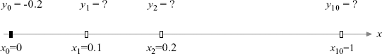
Example 10.1. Given y' = x cos 2y for 0 ≤ x ≤ 1 with h = Δx = 0.1 and y(0) = −0.2, find y(0.1), y(0.2), ..., y(1.0) using the Taylor series method of order 3.

Solution. First, sketch the domain of this problem, as shown in Figure 10.1. We obtain the Taylor series of order 3 as

Equation 10.11. 

The equation requires y, y', y", and y'" in their discrete form. They are evaluated as

Equation 10.12. 

The equations are expressed into their discrete forms as

Equation 10.13. 

Starting at i = 0, we have x₀ = 0 and y₀ = −0.2. The discrete elements become

Equation 10.14. 

We obtain y₁ = y(0.1)

Equation 10.15. 

By repeating the same step above for i = 1 with x₁ = 0.1 and y₁ = −0.195395, we get

Equation 10.16. 

Finally, we obtain the solution:

Equation 10.17. 

The complete results for other values in the range of 0 ≤ x ≤ 1.0 are shown in Table 10.1. Figure 10.2 is the curve representing the solution to the initial-value problem.

Euler's Method

A classic technique called Euler's method is a special case of the Taylor series method whose order is n = 1. The method is derived from the fundamental theorem of calculus, stated as

Equation 10.7. 

Figure 10.2. Solution graph for Example 10.1.

Simplifying the above equation gives

Equation 10.8. 

Euler's method is easy to implement as it involves only the first derivative in the Taylor series. It is not necessary to compute the derivatives of higher orders in this method. However, because of its two-term only expansion in the Taylor series, the results obtained using the Euler's method are not as accurate as the Taylor series method using higher orders.

One difficulty with the Taylor series method is the necessity to evaluate one or higher derivatives of the given expression that may become very tedious and complicated. As a result, the method may not be practical for implementation on the computer as a special routine for evaluating the derivatives has to be developed along with the normal program. This special routine may involve symbolic computation, which is one area of study that requires a good understanding of data structure and numerical database knowledge. Therefore, the Taylor series method is seldom used in most applications for solving the initial-value problems in ODE.

A suitable alternative to the Taylor series method is the Runge-Kutta methods, which were first proposed by the German mathematicians, C. Runge and M. W. Kutta in 1900. Because of its simplicity, the Runge-Kutta method became very popular, and several variations to the original method were produced. The general solution for the explicit ODE is given by

Equation 10.9. 

where n is the order of the Runge-Kutta equation, c_j is the weight, and k_j is the term in the Taylor series expansion of the equation y' = g(x, y). We will discuss the Runge-Kutta of order 2 and 4 methods in this chapter, which has two and four terms in the summation of Equation (10.9), respectively.

Originally, the Runge-Kutta method of order 2 (RK2) is derived from the Taylor series method based on the equation given by

Equation 10.21. 

The above equation simplifies into

Equation 10.10. 

where

Equation 10.11a. 

Equation 10.11b. 

and 0 < r ≤ 1. RK2 is stable and produces reasonably good solutions if the value of r is kept in the given range. The method assumes m equal-width subintervals with h = Δx in x₀ ≤ x ≤ x_m.

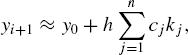
Example 10.2. Solve the problem in Example 10.1 using RK2 with r = 0.8.

Solution. Given

Equation 10.25. 

With r = 0.8,

Equation 10.26. 

This produces

Equation 10.27. 

Continuing at i = 1, we have x₁ = 0.1 and y₁ = −0.195394:

Equation 10.28. 

And, finally,

Equation 10.29. 

Table 10.2 summarizes the results obtained for i = 0, 1, ..., 10.

Heun's Method

Heun's method is a special case of RK2 with r = 1. This produces

Equation 10.12. 

Table 10.2. RK2 solution to the initial-value problem

i	xi	yi	k1	k2
0	0	−0.2	0	0.007368
1	0.1	−0.195394	0.009246	0.016742
2	0.2	−0.181463	0.018697	0.026461
3	0.3	−0.157913	0.028516	0.036621
4	0.4	−0.124331	0.038769	0.047166
5	0.5	−0.080313	0.049356	0.057806
6	0.6	−0.025675	0.059920	0.067932
7	0.7	0.039252	0.069784	0.076593
8	0.8	0.113292	0.077955	0.082625
9	0.9	0.194166	0.083298	0.084967
10	1	0.278508	0.084883	0.083099

where k₁ = hg(x_i, y_i) and k₂ = hg(x_i + h, y_i + k₁). To implement this method, Algorithm 10.2 is used by setting r = 1.

Modified Euler-Cauchy Method

The modified Euler-Cauchy is another special case of RK2 with r = 0.5 to produce

Equation 10.13. 

where k₁ = hg(x_i, y_i) and k₂ = hg(x_i + 0.5h, y_i + 0.5k₁). Although k₁ appears missing in Equation (10.13), the variable is still needed in the evaluation of k₂ and, there-fore, will still need to be evaluated.

The Runge-Kutta method of order 4 (RK4) is derived from the Taylor series of order 4 by approximating the second, third, and fourth derivatives. The method is given as

Equation 10.14. 

where

Equation 10.15a. 

Equation 10.15b. 

Equation 10.15c. 

Equation 10.15d. 

RK4 is a method of choice in many applications for solving the initial-value problem as it provides a more accurate solution compared with RK2. The method is also easy to implement, as summarized in Algorithm 10.3. Example 10.3 shows an example from this method.

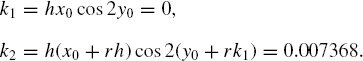
Example 10.3. Solve the problem in Example 10.1 using RK4.

Solution. Given

At i = 0, x₀ = 0 and y₀ = −1. This produces

Equation 10.37. 

Therefore,

Equation 10.38. 

At i = 1, x₀ = 0.1 and y₀ = −0.195386. With similar steps, we get

Equation 10.39. 

The above values produce

Equation 10.40. 

The full results of Example 10.3 are listed in Table 10.3.

All the methods discussed in the earlier sections are single-step methods. The solutions to these methods are based on iterations starting from a single initial value. The results obtained are good, but they may not be precise because of factors such as error truncation and the approximated approach in the methods.

A refinement to the solution in a single-step method is the multistep method. A multistep method implements the predictor-corrector approach, which first deploys a predictor function to predict the solution using the Lagrange polynomial interpolation. The predicted value is then refined further using a corrector function.

We discuss the solution to the first-order ODE problem

Adams-Bashforth-Moulton Method

The Adams-Bashforth-Moulton(ABM) method is the most popular multi step method for solving the initial-value problem. The method is based on the fundamental theorem of calculus from y = f (x) given by

Equation 10.41. 

Table 10.4. Adams-Bashforth predictor functions

Adams-Bashforth	Predictor Function
Two-step
Three-step
Four-step

Table 10.5. Adams-Moulton corrector functions

Adams-Moulton	Corrector Function
Two-step
Three-step

The Adams-Bashforth-Moulton method is a two-fold process consisting of the predictor and corrector functions, p_i+1 and y_i+1. The predictor function is called the Adams-Bashforth function, whereas the corrector is the Adams-Moulton function. Several variations to the method have been documented, and they differ through the number of step sizes in both the predictor and the corrector functions.

Tables 10.4 and 10.5 show some of the most common Adams-Bashforth predictor and Adams-Moulton corrector functions. We discuss the implementation of the Adams-Bashforth-Moulton method using the four-step Adams-Bashforth method as the predictor function and the three-step Adams-Moulton function as the corrector function. The functions are given as

Four-step Adams-Bashforth Equation (Predictor):

Equation 10.16a. 

Three-step Adams-Moulton Equation (Corrector):

Equation 10.16b. 

The Adams-Bashforth predictor is based on the Lagrange polynomial approximation on four points, (x_i−3, y_i−3), (x_i−2, y_i−2), (x_i−1, y_i−1), and (x_i, y_i) to produce the extrapolated point (x_i+1, p_i+1) using Equation (10.16a). Starting with i = 3, the values of g(x₀, y₀), g(x₁, y₁), g(x₂, y₂) and g(x₃, y₃) are first evaluated to produce (x₄, p₄). Any single-step method discussed earlier can be used to evaluate these three values.

The Adams-Moulton corrector involves a Lagrange interpolation over the points (x_i−2, y_i−2), (x_i−1, y_i−1), (x_i, y_i) and the new point (x_i+1, p_i+1) starting at i = 3, to produce the corrected value, (x_i+1, y_i+1). With i = 3, the corrected value of (x₄, y₄) is obtained using Equation (10.16b) from the values of g(x₁, y₁), g(x₂, y₂), and g(x₃, y₃).

Adams-Bashforth-Moulton method.

Given y' = g(x, y), y₀ = f(x₀), h = Δx and m;

For i = 0 to 2

Evaluate y_i+1 using RK2, RK4, or Taylor methods;

Endfor

For i = 3 to m

If i < m

Evaluate p_i+1 using Equation (10.16a);

Evaluate y_i+1 using Equation (10.16b);

Update x_i+1 = x_i + h;

Endfor

Algorithm 10.4 outlines the computational steps for the Adams-Bashforth− Moulton method. This algorithm is illustrated using Example 10.4.

Example 10.4. Solve the problem in Example 10.1 using the Adams-Bashforth-Moulton method, starting with RK4 for the first three values.

Solution. Starting with x₀ = 0 from the initial value, we apply RK4 to produce the values of y₁, y₂, and y₃. The values are obtained from Example 10.3, as

Equation 10.44. 

We get the predictor value at i = 3:

Equation 10.45. 

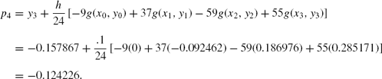
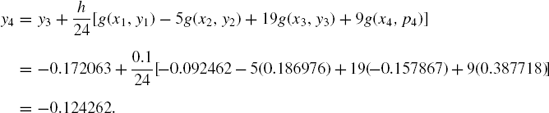
The corrected value follows:

Equation 10.46. 

Table 10.6. Results from Example 10.4

i	xi	pi	yi
0	0		−0.200000
1	0.1		−0.195386
2	0.2		−0.181439
3	0.3		−0.157867
4	0.4	−0.124226	−0.124262
5	0.5	−0.080158	−0.080220
6	0.6	−0.025469	−0.025564
7	0.7	0.039497	0.039375
8	0.8	0.113541	0.113423
9	0.9	0.194379	0.194324
10	1	0.278675	0.278753

Similar calculations for i = 4 produce p₅ and y₅, as follows:

Equation 10.47. 

The full results from Example 10.4 are shown in Table 10.6.

An initial-value problem also arises from a system of ordinary differential equations. A system of first-order ordinary differential equations consists of two or more differential equations that share the same set of variables. As in the system of linear equations, a system with n differential equations requires n initial values before it can be solved with unique solutions.

Definition 10.4. In general, the initial-value problem for a system of n ordinary differential equations involving y₁(x), y₂(x), ..., y_n(x) can be written as

Equation 10.17a. 

where g₁(x, y₁, y₂, ..., y_n), g₂(x, y₁, y₂, ..., y_n), ..., g_n(x, y₁, y₂, ..., y_n) are the given functions in x₀ ≤ x ≤ x_m. The initial values in this problem are given by

Equation 10.17b. 

The domain for this problem consists of the successive points x₀, x₁, ..., x_m in m equal-width subintervals that are h = Δx apart.

Primarily, the solution to an initial-value problem involving a system of differential equations is derived from the same methods used in the single-equation case. Therefore, any method discussed earlier can be applied to solve this problem.

We discuss the Runge-Kutta of order 4 method for solving a system of two differential equations having three variables each. A system of two differential equations with three variables x, y(x), and z(x) in x₀ ≤ x ≤ x_m has the following form:

Equation 10.50. 

The initial values are given by y₀ = y(x₀) and z₀ = z(x₀). The discrete values of x are expressed as x_i for i = 0, 1, 2, ..., m. Since the intervals are uniform with width h= Δx, the terms in x can be expressed as

Equation 10.51. 

The RK4 method for a system of two differential equations is expressed as

Equation 10.18a. 

Equation 10.18b. 

In Equations (10.18a) and (10.18b), k_i and K_i for i = 1, 2, 3, 4 are the RK4 parameters defined in Equations (10.15a), (10.15b), (10.15c), and (10.15d). They are

Equation 10.54. 

Algorithm 10.5 summarizes the steps in solving the initial-value problem from a system of two ordinary differential equations using RK4.

System of first-order ODE with variables using RK4.

Given

Given the initial values, y₀ = y(x₀) and z₀ = z(x₀);

For i = 0 to m

Evaluate k₁ = hg₁ (x_i, y_i, z_i);

Evaluate K₁ = hg₂(x_i, y_i, z_i);

Evaluate k₂ = hg₁(x_i + h/2, y_i + k₁/ 2, z_i + K₁/2);

Evaluate K₂ = hg₂(x_i + h/2, y_i + k₁/2, z_i + K₁/2);

Evaluate k₃ = hg₁(x_i + h/2, y_i + k₂/ 2, z_i + K₂/ 2);

Evaluate K₃ = hg₂(x_i + h/2, y_i + k₂/ 2, z_i + K₂/2);

Evaluate k₄ = hg₁(x_i + h, y_i + k₃, z_i + K₃);

Evaluate K₄ = hg₂(x_i + h, y_i + k₃, Z_i + K₃).

If i < m

Compute y_i+1 using Equation (10.18a);

Compute z_i+1 using Equation (10.18b);

Update x_i+1 ← x_i + h;

Endif

Endfor

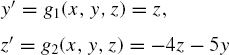
Example 10.5. Solve the differential equations

Solution. The system consists of

Equation 10.55. 

We obtain m = (x_m − x₀)/h = (1 − 0)/ 0.1 = 10. The parameters in RK4 are evaluated as

Equation 10.56. 

Therefore,

Equation 10.57. 

Table 10.7 summarizes the results for (x_i, y_i, z_i) for i = 0, 1, ..., 10.

The second-order ordinary differential equation is an equation that has the second derivative as its highest derivative. The general form of a second-order ODE involving y(x) is

Equation 10.19. 

Two problems arise in the second-order ODE, and they are called the initial-value problem and the boundary-value problem. For an interval defined as a ≤ x ≤ b, the initial-value problem involves Equation (10.19) with its initial values at x = a given. A boundary-value problem has its boundary values given at x = a and x = b for solving Equation (10.19).

In solving a second-order ODE problem, conditions from either its initial values or boundary values are needed. A solution obtained from the second-order differential equations may exist uniquely or infinitely. The following theorems describe the cases of unique solution.

Theorem 10.2. Given y" = f(x, y, y') for x₀ ≤ x ≤ x_m with y(x₀) = y₀ and y(x_m) = y_m, which is continuous in

Theorem 10.3. If y" = p(x)y' + q(x)y + r(x) for x₀ ≤ x ≤ x_m, with y(x₀) = y₀ and y(x_m = y_m; p(x), q(x), and r(x) are continuous in [x₀, x_m]; and q(x) > 0 in [x₀, x_m], then the solution is unique.

We discuss the solution to the initial-value problem in the second-order ordinary differential equation using a technique of reducing its order to a system of first-order equations. This is followed by the boundary-value problem involving a method called finite-difference.

The initial-value problem for a second-order ordinary differential equation is defined as follows:

Definition 10.5. The initial-value problem for a continuous second-order ordinary differential equation in an interval defined as x₀ ≤ x ≤ x_m with the variables y = f(x) consists of solving Equation (10.19) with the initial conditions given by

Equation 10.20a. 

Equation 10.20b. 

A second-order ODE requires two initial conditions, one from the normal starting value and another involving the first derivative. One good strategy for solving the initial-value problem for the second-order ODE is to reduce its order to a system of first-order ODEs. The same technique discussed in Section 10.8 can then be applied to solve the problem once the system of first-order ODEs has been obtained. To achieve this objective, any single-step method discussed in this chapter can be used to generate the solution.

We discuss the reduction of the second-order ODE into a system of first-order ODEs. The numerical solution to the initial-value problem involving the second-order ODE can be modeled as the discrete points (x_i, y_i) over m uniform intervals in x₀ ≤ x ≤ x_m whose width is given by h = Δx.

A second-order ODE with two variables, x and y = f(x), can be reduced into a system of two first-order ODEs. This is possible by setting z = y', and this transforms y" into z'. Hence, g(x, y, y', y") = 0 is reduced to the following system of first-order ODEs:

Equation 10.61. 

The initial-value conditions for this problem become y(x₀) = y₀ and z₀ = y'(x₀). The solutions are then obtained by applying the same method discussed in Section 10.8. Any suitable first-order method such as RK2 and RK4 can be used to solve the system of differential equations.

Algorithm 10.6 summarizes the steps in solving the initial-value problem. The method applies RK4 for solving the system of first-order ODEs. The algorithm is illustrated using Example 10.6.

Second-order ODE reduction to first-order ODE system.

Given g(x, y, y', y") = 0, y₀ = y(x₀), y'(x₀) = z₀, h = Δx and m;

Let z = y and z = y";

Form a system with z = y' = g₁(x, y, z) and z' = y" = g₂(x, y, z);

For i = 0 to m

Evaluate k₁ = hg₁(x_i, y_i, z_i);

Evaluate K₁ = hg₂(x_i, y_i, z_i);

Evaluate

Evaluate

Evaluate

Evaluate

Evaluate

Evaluate

If i < m

Compute y_i+1 using Equation (10.18a);

Compute z_i+1 using Equation (10.18b);

Update x_i+1 ← x_i + h;

Endif

Endfor

Example 10.6. Solve the equation y" + 4y' + 5y = 0, with the initial conditions given by y(0) = −1 dan y'(0) = 2, for 0 ≤ x ≤ 1 and h = 0.1.

Solution. The number of subintervals is m = (1 − 0)/0.1 = 10. Let z = y', and this reduces y" + 4y' + 5y = 0 into z' + 4z + 5y = 0. We obtain a system of first-order ODEs, as follows:

Equation 10.62. 

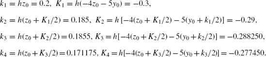
The initial values are y₀ = y(0) = −1 and z₀ = z(0) = 2. The parameters in RK4 are obtained as follows:

Equation 10.63. 

At i = 0, x₀ = 0, y₀ = −1, and z₀ = 2. This gives

Equation 10.64. 

We obtain the first solution as

Equation 10.65. 

The full results from this problem are shown in Table 10.8.

The boundary-value problem for a second-order ordinary differential equation has the boundary conditions given. In an interval defined as a ≤ x ≤ b, the boundaries for the continuous function y = f(x) in the interval are the left and right points, (a, f(a)) and (b, f(b)). To solve the differential equation, the boundary values must be given.

A boundary is an end point in the given interval or domain of the problem. There are two types of boundaries in an ordinary differential equation:

We will deal with the first type of boundary condition in this section and with the second type in the next section.

Definition 10.6. The boundary-value problem involving a second-order ordinary differential equation is Equation (10.19) in x₀ ≤ x ≤ x_m with boundary conditions given by y(x₀) = y₀ and y(x_m) = y_m. In this interval, the width is given by h = Δx and there are m uniform subintervals.

We restrict our discussion on the boundary-value problems to the case of linear second-order ODEs. A second-order differential equation is said to linear if it can be expressed into the following form:

Equation 10.21. 

where p(x), q(x), r(x), and w(x) are continuous functions of x in the interval x₀ ≤ x ≤ x_m.

A common approach for solving a linear second-order differential equation with boundary conditions is the finite-difference method. The method is based on the approximation of the derivatives of y at several finite points in the interval to yield a finite-difference formula. The points are distributed at equal-width subintervals so that the derivatives y' and y" can be replaced by their approximated discrete values.

The solution to the boundary-value problem for ODE2 consists of two main steps, as depicted in Figure 10.3. First, the differential equation is discretized where the terms involving y' and y" are replaced by their approximated values using the central-difference rules. This step leads the way to the formation of the finite-difference formula for the problem.

The second step starts by applying the finite-difference formula to the m subintervals in x₀ ≤ x ≤ x_m. The finite-difference formula is applied at each of the m − 1 interior points in the interval to produce a system of (m − 1) × (m − 1) linear equations. A technique from Chapter 5, such as the Gaussian elimination method, is then applied to solve this system to produce the final solution to the boundary-value problem.

Algorithm 10.7 outlines the implementation of the finite-difference method for solving the boundary-value problem for a linear second-order ODE.

Figure 10.3. Two-step solution to the boundary value problem in the second-order ODE.

We discuss the general solution to Equation (10.21) using Algorithm 10.7. The discrete form of this equation is given by

Equation 10.67. 

Let p_i = p(x_i), q_i = q(x_i), r_i = r(x_i), and w_i = w(x_i), and the above equation becomes

Equation 10.68. 

Finite-difference values are obtained by employing the central difference rules discussed in Chapter 8 to approximate the first and second derivatives, given as

Equation 10.69. 

Substituting y' and y", we get

Equation 10.70. 

Rearranging the terms in the order of y_i−1, y_i and y_i+1, we obtain the finite-difference formula for the given problem:

Equation 10.22. 

There are m − 1 unknowns in the system, y_i for i = 1, 2, ..., m − 1, which can be solved from the (m − 1) × (m − 1) system of linear equations. This system of linear equations is obtained by first substituting i = 1, 2, ..., m − 1 into the above equation. The process starts with i = 1:

Equation 10.72. 

Since the value of y₀ is given, the first term above is moved to the right-hand side of the equation to give

Equation 10.73. 

At i = m − 1, the equation becomes

Equation 10.74. 

Since the value of y_m is given, the last term in the left-hand side is moved to the right-hand side, and this produces the last equation in the system as

Equation 10.75. 

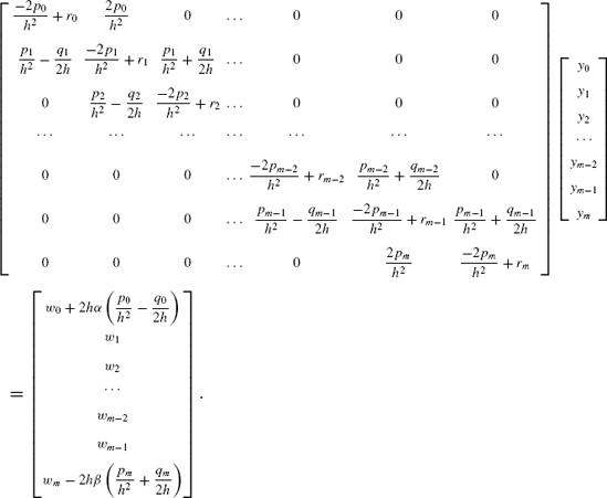
Regrouping all the above equations into a matrix form, we obtain a tridiagonal system of linear equations of size (m − 1) × (m − 1), as follows:

Equation 10.23. 

From the above system of linear equations, we obtain the algorithm for the nonzero entries of A = [a_i,j] and b = [b_i] in Ay = b, as follows:

Equation 10.24a. 

Equation 10.24b. 

Since Equation (10.23) is tridiagonal, the most practical approach for solving this system is the Thomas algorithm as the computational steps required in this method are not as massive as in other methods. We discuss an example that shows the method for solving this problem.

Figure 10.4. The solution diagram for Example 10.7.

Example 10.7. Given (cosx)y" + (sin(2x − 1)) y' + (sin(1 − 5x))y = x cosx in 1 < x < 3 whose width is h = Δx = 0.4, the boundary values in this problem are given as y(1) = −1 and y(3) = 1. Find the values of y(1.4), y(1.8), y(2.2), and y(2.6).

Solution. Figure 10.4 shows the solution diagram for the problem. There are four unknowns in this problem, y_i for i = 1, 2, 3, 4, since m = 5. We start with

Equation 10.79. 

Applying the central-difference rules for substituting y'_i and y"_i,

Equation 10.80. 

Simplifying the terms in the above equation, we obtain the following finite-difference formula:

Equation 10.81. 

The next step is to form the system of linear equations. A system of four linear equations is to be formed since there are four unknowns, y₁, y₂, y₃, and y₄. The equations are found by setting i = 1, 2, 3, 4 into the finite-difference formula to form a 4 × 4 system of linear equations, as follows:

Equation 10.82. 

Figure 10.5. Solution curve for Example 10.7.

In matrix form, the linear equations become

Equation 10.83. 

The above system of linear equations is solved to produce the following solution:

Equation 10.84. 

Figure 10.5 shows the solution graph for Example 10.7.

Under certain circumstances, the boundary conditions for the second-order ODE in Equation (10.21) may be given in the form of derivatives, as follows:

Equation 10.85. 

where α and β are constants and m is the number of subintervals in x₀ ≤ x ≤ x_m.

In solving this problem, similar steps as in the previous case are applied to obtain the finite-difference formula in Equation 10.22.

Equation 10.86. 

The left boundary is y'₀ = α. Applying the central-difference rule from Equation (8.5a),

Equation 10.87. 

We obtain a virtual value, y₋₁ as this quantity is not inside y₀ ≤ y ≤ y_m. Expressing y₋₁ as a subject of the equation, we obtain

Equation 10.88. 

The right boundary condition consists of y'_m = β, which becomes

Equation 10.89. 

Again, another virtual value y_m+1 is obtained as it is outside of y₀ ≤ y ≤ y_m. This value is made the subject, as follows:

Equation 10.90. 

It can be verified that the virtual values are only applicable in the finite-difference formula in cases of i = 0 and i = m. At i = 0, Equation (10.22) produces:

Equation 10.91. 

Substituting the value of y₋₁, the above equation simplifies to

Equation 10.25. 

Similarly, applying Equation (10.22) at i = m:

Equation 10.93. 

Substituting the value of y_m+1:

Equation 10.26. 

For i = 1, 2, ..., m − 1, the entries in each row of the coefficient matrix consist of the diagonal, and its left and right terms, as follows:

Equation 10.95. 

We obtain a (m + 1) × (m + 1) tridiagonal system of linear equations:

Equation 10.27. 

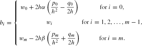
Equation (10.27) is summarized as Ay = b, where A = [a_ij] is the coefficient matrix in the left-hand side, b = [b_i] is the vector in the right side of the equation, and y = [y_i] is the unknown vector, for i, j = 0, 1, 2, ..., m. The tridiagonal elements of A are obtained as

Equation 10.28a. 

Equation 10.28b. 

Equation 10.28c. 

From the same equation, we obtain the representation for b, as follows:

Equation 10.28d. 

Collectively, Equations (10.28a), (10.28b), (10.28c), and (10.28d) are sufficient to solve for y. Since the coefficient matrix in Equation (10.27) is tridiagonal, the most suitable choice for solving the system of linear equations is the Thomas algorithm method.

Example 10.8. Given

Solution. There are

Figure 10.6. Graphical representation of the problem.

Equation 10.101. 

Replacing y'_i and y"_i in the above equation using central-difference rules, we get

Equation 10.102. 

The above equation is simplified to produce the finite-difference formula given by

Equation 10.103. 

The boundary values at x₀ = 0 and x₅ in this problem are given in the form of first derivatives at these points. This implies y₀ and y₅ are also the unknowns in this problem along with y₁, y₂, y₃, and y₄. Therefore, there are six unknowns that require the reduction of the boundary-value problem to a 6 × 6 system of linear equations.

The given first derivative at x₀ = 0 is simplified using the central-difference rule to produce a virtual value, y₋₁. This is obtained as follows:

Equation 10.104. 

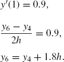
The right boundary value is simplified in a similar fashion to produce another virtual value, y₆, as follows:

Equation 10.105. 

The first virtual value and the finite-difference formula are applied at i = 0 to produce

Equation 10.106. 

Applying the formula at the other interior points produce

Equation 10.107. 

The second virtual value is applied to the right boundary point, at i = 5, to produce

Equation 10.108. 

We obtain the following system of linear equations:

Equation 10.109. 

The above system is solved to produce the final solutions, given by

Equation 10.110. 

The solution curve for this problem is shown in Figure 10.7

Figure 10.7. Solution curve for Example 10.8 in 0 ≤ x ≤ 1.

We discuss the visual interface for the ordinary differential equations problems. The project is called Code10, and it consists of all the methods discussed in this chapter. Code10 is menu-driven, and this provides friendliness to problems that are generally considered difficult.

Figure 10.8 shows the output from Code10, which consists of a menu with eight items that represent the methods in order from top to bottom, as follows: Taylor, Runge-Kutta of order2, Runge-Kutta of order 4, Adams-Bashforth-Moulton, ODE1 system, ODE2 initial-value problem, finite-difference 1, and finite-difference 2. The figure shows the solution to a sample problem from the fifth item in the menu (ODE 1 System), which is an initial-value problem on a system of first-order ODEs given by

Equation 10.111. 

whose initial values are x₀ = 0, y₀ = 0.5, and z₀ = 0.5, for 0 ≤ x ≤ 8. The results are shown in the table with their corresponding graphs of y = q(x) and z = r(x) generated.

Code10 has been designed to allow the user a full control of the input as well as the output. To allow this flexibility, the output from Figure 10.8 is divided into four regions. The first region is the menu displayed as shaded rectangles on the top left. The second region is the input area, which becomes active when an item in the menu is selected. The third region is the list view table for displaying the results from the calculations. The fourth region is the graphical area that displays the solution graph for the problem.

Figure 10.8. An output from Code10.

Code10 has a single class called CCode10, and this class is derived from CFrameWnd. The development files in Code10 are Code10.cpp, Code10.h, and MyParser.obj.

Figure 10.9 is the schematic drawing of Code10 that shows the development stages of Code10. In this diagram, a status flag called fStatus monitors the execution progress whose updated value represents a step in the execution. Initially, fStatus has a value of 0. When an item in the menu is selected, fStatus changes its value to 1. At the same time, a variable called fMenu is assigned with a number that represents the order of the item from top to bottom. The selection also creates edit boxes for collecting input from the user and a push button called Compute that, when activated, calls the function that corresponds to the selected method.

When input has been completed and confirmed with a click at the Compute button, fStatus value is updated to 2. The click causes a call to be made to a function corresponding to the selected method in the menu. This function represents a method for solving the given problem. The function solves the problem according to the input values, and the results are displayed in the list view table through ShowTable(). The solution graph for the problem is also displayed through DrawCurve().

Figure 10.9. Schematic drawing showing the development stages of Code10.

Changes in the input values in the edit boxes are allowed by resetting fStatus to 1 in DrawCurve() once the results have been obtained and displayed. This option is necessary as part of the user-friendliness features for the given problem. With this update, any small changes in the input values will cause the whole data to be reevaluated, and the results are immediately updated both in the table and in the solution graph.

The data structure in Code10 consists of four structures. The first structure is PT, which represents the variables x_i, y_i, p_i, and z_i as the array pt in the methods. The structure also defines the left, right, maximum, and minimum points in the solution curve in the problem. The structure is declared as follows:

typedef struct
{
      double x, y, p, z:  // xi, yi, pi, and zi components
} PT;
PT *pt;

A structure called INPUT declares the input objects, and these objects are linked to an array called input. The structure is declared as

typedef struct
{
      CString item, label,;   // input string and its label
      CPoint hm;          // home coordinates
      CEdit ed;          // edit box
      CRect rc;          // rectangular object
} INPUT;
INPUT input[maxInput+1];

The third structure is MENU, which declares objects for the items in the menu. This structure is declared as

typedef struct
{
      CString item;  // menu item
      CPoint hm;    // home coordinates
      CRect rc;    // rectangular region
} MENU;
MENU menu[nMenuItems+1];

The last structure is CURVE, which provides objects for creating the solution curve. The structure defines the rectangular region for displaying the solution graph.

typedef struct
{
      CRect rc;     // rectangular region
      CPoint hm, end;  // starting and end
              coordinates
} CURVE;
CURVE curve;

Three events are mapped in Code10, namely, the display update, left-button click, and push button click.

BEGIN MESSAGE MAP(CCode10, CFrameWnd)
    ON_WM_PAINT()
    ON_WM_LBUTTONDOWN()

ON_BN_CLICKED(IDC_BUTTON, OnButton)
END_MESSAGE_MAP()

Eight items in the menu represent eight different methods for solving the initial-and boundary-value problems. Each method is represented by a function as described in Table 10.9.

Taylor Series of Order 3 Solution

The Taylor series method is represented by ODE1Taylor(). This function supports the Taylor series method of order three only. It would be a good challenge for the reader to modify the item to make it more flexible by supporting the method using any high order. In the given problem, y = g(x, y) is the input function. Because of the non-symbolic nature of the application, the program does not evaluate the second or third derivatives automatically from the input function. The user needs to enter the derivatives in the edit boxes, and the string will then be passed to parse() for processing.

In reading the input string, the derivatives are represented as single characters in parse(), as follows:

Equation 10.112. 

The representation is necessary so as to use the character codes defined in Table 4.1 where the corresponding codes for x, y, u, v, w, and z are 23, 24, 20, 21, 22, and 25, respectively. For example, y"' = 3xy' − 4(y")² cosxy" is written as

The Taylor series method in ODE1Taylor() is written based on Algorithm 10.1 and Equation (10.6). The function is given as follows:

void CCode10::ODE1Taylor()
{
      double psv[6], tmp, max;
      int psi[6];
      int i;
      double h, u, v, w, z;

      pt[0].x=atof(input[2].item);
      pt[0].y=atof(input[5].item);
      h=atof(input[4].item);
      tmp=atof(input[3].item);
      m=(tmp-pt[0].x)/h; m=((m<M)?m:M);
      max=pt[0].x+(double)m*h;
      tmp=(tmp<max)?tmp:max;
      pt[m].x=tmp;
      psi[1]=23;
      psi[2]=24;
      psi[3]=20;
      psi[4]=21;
      for (i=0;i<=m;i++)
      {
            psv[1]=pt[i].x;
            psv[2]=pt[i].y;
            u=parse(input[1].item, 2, psv, psi);
            psv[3]=u;
            v=parse(input[6].item, 3, psv, psi);
            psv[4]=v;
            w=parse(input[7].item, 4, psv, psi);
            if (i<m)
            {
                 pt[i+1].y=pt[i].y+h*u+pow(h, 2)/
                           2*v+pow(h, 3)/6*w;
                 pt[i+1].x=pt[i].x+h;
            }
       }
}

There are m subintervals that require m iterations for computing y_i, for i = 1, 2, ..., m. The input strings for the equations are read as input[1].item, input[6].item, and input[7].item. These strings are passed to parse() for processing. The returned values are stored as u, v, and w, which represent y', y", and y"', respectively.

psv[1]=pt[i].x;
psv[2]=pt[i].y;
u=parse(input[1].item, 2, psv, psi);
psv[3]=u;
v=parse(input[6].item, 3, psv, psi);
psv[4]=v;
w=parse(input[7].item, 4, psv, psi);

The Taylor series method solves the initial-value problem according to Equation (10.6). The code for this equation is written as

if (i<m)
{
      pt[i+1].y=pt[i].y+h*u+pow(h, 2)/2*v+pow(h, 3)/6*w;
      pt[i+1].x=pt[i].x+h;
}

void CCode10::ODE1RK2()
{
      int i, psi[6];
      double h, r, psv[6], tmp, max;
      double k1, k2;
      pt[0].x=atof(input[2].item);
      pt[0].y=atof(input[5].item);
      h=atof(input[4].item);
      tmp=atof(input[3].item);
      m=(tmp-pt[0].x)/h; m=((m<M)?m:M);
      max=pt[0].x+(double)m*h;
      tmp=(tmp<max)?tmp:max;
      pt[m].x=tmp;
      r=atof(input[6].item);
      psi[1]=23; psi[2]=24;
      for (i=0;i<=m;i++)
      {

psv[1]=pt[i].x;
      psv[2]=pt[i].y;
      k1=h*parse(input[1].item, 2, psv, psi);
      psv[1]=pt[i].x+r*h;
      psv[2]=pt[i].y+r*k1;
      k2=h*parse(input[1].item, 2, psv, psi);
      if (i<m)
      {
            pt[i+1].y=pt[i].y+(1-1/(2*r))*k1+1/(2*r)*k2;
            pt[i+1].x=pt[i].x+h;
      }
   }
}

psv[1]=pt[i].x;
psv[2]=pt[i].y;
k1=h*parse(input[1].item, 2, psv, psi);
psv[1]=pt[i].x+r*h;
psv[2]=pt[i].y+r*k1;
k2=h*parse(input[1].item, 2, psv, psi);

if (i<m)
{
      pt[i+1].y=pt[i].y+(1-1/(2*r))*k1+1/(2*r)*k2;
      pt[i+1].x=pt[i].x+h;
}

void CCode10::ODE1RK4()
{
      int i, psi[6];
      double h, psv[6], tmp, max;
      double k1, k2, k3, k4;
      pt[0].x=atof(input[2].item);

pt[0].y=atof(input[5].item);
      h=atof(input[4].item);
      tmp=atof(input[3].item);
      m=(tmp-pt[0].x)/h;
      m=((m<M)?m:M);
      max=pt[0].x+(double)m*h;
      tmp=(tmp<max)?tmp:max;
      pt[m].x=tmp;
      psi[1]=23; psi[2]=24;
      for (i=0;i<=m;i++)
      {
            psv[1]=pt[i].x;
            psv[2]=pt[i].y;
            k1=h*parse(input[1].item, 2, psv, psi);

            psv[1]=pt[i].x+h/2;
            psv[2]=pt[i].y+k1/2;
            k2=h*parse(input[1].item, 2, psv, psi);

            psv[1]=pt[i].x+h/2;
            psv[2]=pt[i].y+k2/2;
            k3=h*parse(input[1].item, 2, psv, psi);

            psv[1]=pt[i].x+h;
            psv[2]=pt[i].y+k3;
            k4=h*parse(input[1].item, 2, psv, psi);
            if (i<m)
            {
                  pt[i+1].y=pt[i].y+(k1+2*k2+2*k3+k4)/6;
                  pt[i+1].x=pt[i].x+h;
            }
      }
}

psv[1]=pt[i].x;
psv[2]=pt[i].y;
k1=h*parse(input[1].item, 2, psv, psi);

psv[1]=pt[i].x+h/2;
psv[2]=pt[i].y+k1/2;
k2=h*parse(input[1].item, 2, psv, psi);

psv[1]=pt[i].x+h/2;
psv[2]=pt[i].y+k2/2;
k3=h*parse(input[1].item, 2, psv, psi);

psv[1]=pt[i].x+h;
psv[2]=pt[i].y+k3;
k4=h*parse(input[1].item, 2, psv, psi);

if (i<m)
{
      pt[i+1].y=pt[i].y+(k1+2*k2+2*k3+k4)/6;
      pt[i+1].x=pt[i].x+h;
}

void CCode10::ODE1AB()
{
      int i, psi[6];
      double h, f0, f1, f2, f3, fp, psv[6], tmp, max;
      double k1, k2, k3, k4;
      pt[0].x=atof(input[2].item); pt[0].y=atof(input[5].item);
      h=atof(input[4].item);
      tmp=atof(input[3].item);
      m=(tmp-pt[0].x)/h; m=((m<)?m:M);
      max=pt[0].x+(double)m*h;
      tmp=(tmp<ax)?tmp:max;
      pt[m].x=tmp;
      psi[1]=23; psi[2]=24;
      for (i=0;i<=m;i++)
      {
            if (i<3)
            {
                  psv[1]=pt[i].x;
                  psv[2]=pt[i].y;
                  k1=h*parse(input[1].item, 2, psv, psi);

                  psv[1]=pt[i].x+h/2;

psv[2]=pt[i].y+k1/2;
                  k2=h*parse(input[1].item, 2, psv, psi);

                  psv[1]=pt[i].x+h/2;
                  psv[2]=pt[i].y+k2/2;
                  k3=h*parse(input[1].item, 2, psv, psi);

                  psv[1]=pt[i].x+h;
                  psv[2]=pt[i].y+k3;
                  k4=h*parse(input[1].item, 2, psv, psi);

                  pt[i+1].y=pt[i].y+(k1+2*k2+2*k3+k4)/6;
            }
            if (i<)
            {
                  pt[i+1].x=pt[i].x+h;
                  if (i>=3)
                  {
                        psv[1]=pt[i-3].x;
                        psv[2]=pt[i-3].y;
                        f0=parse(input[1].item, 2, psv, psi);

                        psv[1]=pt[i-2].x;
                        psv[2]=pt[i-2].y;
                        f1=parse(input[1].item, 2, psv, psi);

                        psv[1]=pt[i-1].x;
                        psv[2]=pt[i-1].y;
                        f2=parse(input[1].item, 2, psv, psi);

                        psv[1]=pt[i].x;
                        psv[2]=pt[i].y;
                        f3=parse(input[1].item, 2, psv, psi);
                        pt[i+1].p=pt[i].y+h/24*(−9*f0+37*f1
                                  −59*f2+55*f3);

                        psv[1]=pt[i+1].x;
                        psv[2]=pt[i+1].p;
                        fp=parse(input[1].item, 2, psv, psi);
                        pt[i+1].y=pt[i].y+h/24*(f1-5*f2+19*f3
                                  +9*fp);
                  }
           }
      }
}

if (i<3)
{
      psv[1]=pt[i].x;
      psv[2]=pt[i].y;
      k1=h*parse(input[1].item, 2, psv, psi);

      psv[1]=pt[i].x+h/2;
      psv[2]=pt[i].y+k1/2;
      k2=h*parse(input[1].item, 2, psv, psi);

      psv[1]=pt[i].x+h/2;
      psv[2]=pt[i].y+k2/2;
      k3=h*parse(input[1].item, 2, psv, psi);

     psv[1]=pt[i].x+h;
     psv[2]=pt[i].y+k3;
     k4=h*parse(input[1].item, 2, psv, psi);

     pt[i+1].y=pt[i].y+(k1+2*k2+2*k3+k4)/6;
}

if (i<m)
{
      pt[i+1].x=pt[i].x+h;
      if (i>=3)
      {
            psv[1]=pt[i-3].x;
            psv[2]=pt[i-3].y;
            f0=parse(input[1].item, 2, psv, psi);

            psv[1]=pt[i-2].x;
            psv[2]=pt[i-2].y;
            f1=parse(input[1].item, 2, psv, psi);

            psv[1]=pt[i-1].x;
            psv[2]=pt[i-1].y;
            f2=parse(input[1].item, 2, psv, psi);

            psv[1]=pt[i].x;

psv[2]=pt[i].y;
            f3=parse(input[1].item, 2, psv, psi);
            pt[i+1].p=pt[i].y+h/24*(−9*f0+37*f1-59*f2+55*f3);

            psv[1]=pt[i+1].x;
            psv[2]=pt[i+1].p;
            fp=parse(input[1].item, 2, psv, psi);
            pt[i+1].y=pt[i].y+h/24*(f1-5*f2 +19*f3+9*fp);
      }
}

void CCode10::ODE1System()
{
      int i, psi[6];
      double h, psv[6], tmp, max;
      double k1, k2, k3, k4;
      double K1, K2, K3, K4;
      pt[0].x=atof(input[3].item);
      pt[0].y=atof(input[4].item);
      pt[0].z=atof(input[5].item);
      h=atof(input[6].item);
      tmp=atof(input[7].item);
      m=(tmp-pt[0].x)/h; m=((m<M)?m:M);
      max=pt[0].x+(double)m*h;
      tmp=(tmp<Max)?tmp:max;
      pt[m].x=tmp;
      psi[1]=23; psi[2]=24; psi[3]=25;
      for (i=0;i<=m;i++)
      {
            psv[1]=pt[i].x;
            psv[2]=pt[i].y;
            psv[3]=pt[i].z;
            k1=h*parse(input[1].item, 3, psv, psi);

K1=h*parse(input[2].item, 3, psv, psi);

            psv[1]=pt[i].x+h/2;
            psv[2]=pt[i].y+k1/2;
            psv[3]=pt[i].z+K1/2;
            k2=h*parse(input[1].item, 3, psv, psi);
            K2=h*parse(input[2].item, 3, psv, psi);

            psv[1]=pt[i].x+h/2;
            psv[2]=pt[i].y+k2/2;
            psv[3]=pt[i].z+K2/2;
            k3=h*parse(input[1].item, 3, psv, psi);
            K3=h*parse(input[2].item, 3, psv, psi);

            psv[1]=pt[i].x+h;
            psv[2]=pt[i].y+k3;
            psv[3]=pt[i].z+K3;
            k4=h*parse(input[1].item, 3, psv, psi);
            K4=h*parse(input[2].item, 3, psv, psi);

            if (i<m)
            {
                  pt[i+1].y=pt[i].y+(k1+2*k2+2*k3+k4)/6;
                  pt[i+1].z=pt[i].z+(K1+2*K2+2*K3+K4)/6;
                  pt[i+1].x=pt[i].x+h;
            }
      }
}

void CCode10::ODE2toODE1System()
{
      int i, psi[6];
      double psv[6];
      double h, tmp;

double k1, k2, k3, k4;
      double K1, K2, K3, K4;
      pt[0].x=atof(input[2].item);
      pt[0].y=atof(input[3].item);
      pt[0].z=atof(input[4].item);
      h=atof(input[5].item);
      tmp=atof(input[6].item);
      m=(tmp-pt[0].x)/h; m=((m<M)?m:M);
      pt[m].x=tmp;
      psi[1]=23; psi[2]=24; psi[3]=25;
      for (i=0;i<=m;i++)
      {
            psv[1]=pt[i].x;
            psv[2]=pt[i].y;
            psv[3]=pt[i].z;
            k1=h*pt[i].z; K1=h*parse(input[1].item, 3, psv, psi);

            psv[1]=pt[i].x+h/2;
            psv[2]=pt[i].y+k1/2;
            psv[3]=pt[i].z+K1/2;
            k2=h*(pt[i].z+K1/2); K2=h*parse(input[1].item, 3,
                    psv, psi);

            psv[1]=pt[i].x+h/2;
            psv[2]=pt[i].y+k2/2;
            psv[3]=pt[i].z+K2/2;
            k3=h*(pt[i].z+K2/2); K3=h*parse(input[1].item,
                  3, psv, psi);

            psv[1]=pt[i].x+h;
            psv[2]=pt[i].y+k3;
            psv[3]=pt[i].z+K3;
            k4=h*(pt[i].z+K3); K4=h*parse(input[1].item,
                  3, psv, psi);

            if (i<m)
            {
                  pt[i+1].y=pt[i].y+(k1+2*k2+2*k3+k4)/6;
                  pt[i+1].z=pt[i].z+(K1+2*K2+2*K3+K4)/6;
                  pt[i+1].x=pt[i].x+h;
            }
      }
}

void CCode10::ODE2FD1()
{
      int i, j, psi[6];
      double psv[6], h, tmp;
      double **a, *b;
      double *p, *q, *r, *w;
      b=new double [M+1];
      p=new double [M+1];
      q=new double [M+1];
      r=new double [M+1];
      w=new double [M+1];
      a=new double *[M+1];
      h=atof(input[5].item);
      m=(int)(atof(input[7].item)-atof(input[6].item))/h;
              m=((m<M)?m:M);
      pt[0].x=atof(input[6].item);
      pt[m].x=pt[0].x+(double)m*h;
      pt[0].y=atof(input[8].item);
      pt[m].y=atof(input[9].item);
      psi[1]=23;
      for (i=1;i<=m-1;i++)
      {
            pt[i].x=pt[i-1].x+h;
            psv[1]=pt[i].x;
            p[i]=parse(input[1].item, 1, psv, psi);
            q[i]=parse(input[2].item, 1, psv, psi);
            r[i]=parse(input[3].item, 1, psv, psi);
            w[i]=parse(input[4].item, 1, psv, psi);
      }
      for (i=0;i<=M;i++)
            a[i]=new double [M+1];
      for (i=1;i<=m-1;i++)
      {
            for (j=1;j<=m-1;j++)
                  a[i][j]=0;
            b[i]=0;
      }
      b[1]=w[1]-(p[1]/(h*h)-q[1]/(2*h))*pt[0].y;

b[m-1]=w[m-1]-(p[m-1]/(h*h)+q[m-1]/(2*h))*pt[m].y;
      for (i=1;i<=m-1;i++)
      {
            a[i][i]=−2*p[i]/(h*h)+r[i];
            if (i<m-1)
                  a[i+1][i]=p[i+1]/(h*h)-q[i+1]/(2*h);
            if (i>1)
                  a[i-1][i]=p[i-1]/(h*h)+q[i-1]/(2*h);
            if (i>1 && i<m-1)
                  b[i]=w[i];
      }
      SolveSLE(a, b);
      for (i=0;i<=M;i++)
            delete a[i];
      delete p, q, r, w, a, b;
}

psi[1]=23;
for (i=1;i<=m-1;i++)
{
      pt[i].x=pt[i-1].x+h;
      psv[1]=pt[i].x;
      p[i]=parse(input[1].item, 1, psv, psi);
      q[i]=parse(input[2].item, 1, psv, psi);
      r[i]=parse(input[3].item, 1, psv, psi);
      w[i]=parse(input[4].item, 1, psv, psi);
}

for (i=1;i<=m-1;i++)
{
      for (j=1;j<=m-1;j++)
      a[i][j]=0;
      b[i]=0;
}

b[1]=w[1]-(p[1]/(h*h)-q[1]/(2*h))*pt[0].y;
b[m-1]=w[m-1]-(p[m-1]/(h*h)+q[m-1]/(2*h))*pt[m].y;
for (i=1;i<=m-1;i++)
{
      a[i][i]=−2*p[i]/(h*h)+r[i];
      if (i<m-1)
            a[i+1][i]=p[i+1]/(h*h)-q[i+1]/(2*h);
      if (i>1)
            a[i-1][i]=p[i-1]/(h*h)+q[i-1]/(2*h);
      if (i>1 && i<m-1)
            b[i]=w[i];
}

void CCode10::SolveSLE(double **a, double *b)
{
      int i, j, k, lo, hi;
      double m1, Sum;
      if (fMenu==7)
      {
            lo=1; hi=m-1;
      }
      if (fMenu==8)
      {
            lo=0; hi=m;
      }
      for (k=lo;k<=hi-1;k++)
            for (i=k+1;i<=hi;i++)
            {
                  m1=a[i][k]/a[k][k];
                  for (j=lo;j<=hi;j++)
                        a[i][j] -= m1*a[k][j];
                  b[i] -= m1*b[k];
            }
      for (i=hi;i>=lo;i--)
      {
            Sum=0;
            pt[i].y=0;
            for (j=i;j<=hi;j++)

Sum += a[i][j]*pt[j].y;
            pt[i].y=(b[i]-Sum)/a[i][i];
      }
}

void CCode10::ODE2FD2()
{
      int i, j, psi[6];
      double psv[6], tmp;
      double h, alpha, beta;
      double **a, *b;
      double *p, *q, *r, *w;
      b=new double [M+1];
      p=new double [M+1];
      q=new double [M+1];
      r=new double [M+1];
      w=new double [M+1];
      a=new double *[M+1];
      for (i=0;i<=M;i++)
            a[i]=new double [M+1];
      h=atof(input[5].item);
      m=(int)(atof(input[7].item)-atof(input[6].item))/h;
              m=((m<M)?m:M);
      pt[0].x=atof(input[6].item);
      pt[m].x=pt[0].x+(double)m*h;
      alpha=atof(input[8].item); beta=atof(input[9].item);
      for (i=0;i<=m;i++)
      {
            if (i<m)
                  pt[i+1].x=pt[i].x+h;

psv[1]=pt[i].x; psi[1]=23;
                  p[i]=parse(input[1].item, 1, psv, psi);
                  q[i]=parse(input[2].item, 1, psv, psi);
                  r[i]=parse(input[3].item, 1, psv, psi);
                  w[i]=parse(input[4].item, 1, psv, psi);
      }
      for (i=0;i<=m;i++)
      {
            for (j=0;j<=m;j++)
                  a[i][j]=0;
            b[i]=0;
      }
      for (i=0;i<=m;i++)
      {
            a[i][i]=−2*p[i]/(h*h)+r[i];
            if (i>0 && i<M)
                  a[i][i+1]=p[i]/(h*h)+q[i]/(2*h);
            if (i<m-1)
                  a[i+1][i]=p[i+1]/(h*h)-q[i+1]/(2*h);
            if (i>0 && i<M)
                  b[i]=w[i];
      }
      a[0][1]=2*p[0]/m;
      a[m][m-1]=2*p[m]/(h*h);
      b[0]=w[0]+(p[0]/(h*h)-q[0]/(2*h))*2*h*alpha;
      b[m]=w[m]-(p[m]/(h*h)+q[m]/(2*h))*2*h*beta;
      SolveSLE(a, b);
      for (i=0;i<=M;i++)
            delete a[i];
      delete p, q, r, w, a, b;
}

for (i=0;i<=m;i++)

{
      a[i][i]=−2*p[i]/(h*h)+r[i];
      if (i>0 && i<M)
            a[i][i+1]=p[i]/(h*h)+q[i]/(2*h);
      if (i<m-1)
            a[i+1][i]=p[i+1]/(h*h)-q[i+1]/(2*h);
      if (i>0 && i<m)
            b[i]=w[i];
}
a[0][1]=2*p[0]/m;
a[m][m-1]=2*p[m]/(h*h);
b[0]=w[0]+(p[0]/(h*h)-q[0]/(2*h))*2*h*alpha;
b[m]=w[m]-(p[m]/(h*h)+q[m]/(2*h))*2*h*beta;

The chapter discusses the numerical solutions to the first- and second-order ordinary differential equations. The first-order differential equations involve initial-value problems, and their numerical solutions consist of the Taylor series, Runge-Kutta of order 2, Runge-Kutta of order 4, and the Adam-Bashforth-Moulton methods. Problems in the second-order ordinary differential equations include both the initial-value and boundary-value problems. Their initial-value solutions are derived from the first-order methods, whereas the boundary-value problems are solved using the finite-difference methods.

Several creative projects can be embarked from our discussion. Problems in ordinary differential equations are commonly encountered in science and engineering. The problems are expressed in the form of models involving ordinary differential equations, whereas simulations are performed to support these theoretical models. In most cases, visualization from the solution is necessary to support the work. Therefore, programming with a friendly graphical user interface is needed for visualizing the results from the applications.

The following exercises are intended to test your understanding of the materials discussed in this chapter. Use six decimal places for calculations.