
The eigenvalues of a square matrix are important parameters in determining things like the stability of the structure where the matrix is based. A bridge depends on the strength of its beam across a given length whose stability is determined by its eigenvalues. In image processing, the eigenvalues of a matrix that represent an image hold the key to the quality of the image. With a proper technique, a blur image can be transformed into a crisp one once the eigenvalues of its corresponding matrix are known.
Therefore, finding the eigenvalues of a square matrix and their corresponding eigenvectors has become an important problem in many applications. The eigenvalue problem can be stated as follows:
Given a matrix A, find the nonzero vectors v such that Av = λ v, where λ is the eigenvalue and v is its corresponding eigenvector. The real eigenvalues and its eigenvectors of the matrix will not exist if no value of v can satisfy Av = λv.
In many applications, it may not be necessary to find all the eigenvalues of a given matrix. In this case, the eigenvalues whose values are extreme become the focus. An eigenvalue whose modulus is the largest is called the most dominant eigenvalue, whereas one that is smallest is called the least dominant eigenvalue. In most applications, it may not be necessary to find all the eigenvalues of a given matrix. Finding the most dominant eigenvalue or the least dominant eigenvalue may be sufficient in providing the solution to a given problem.
We discuss two iterative methods called the power method and the shifted power method, for finding the most dominant and least dominant eigenvalues of a matrix, respectively.
In a transformation, an eigenvector is a nonzero vector v, which transforms the given quantity A into a new vector b that has the same direction as v. This transformation can be written as T [v] = λ v = b or
In the above equation, λ is the scale factor for this transformation, and it is called the eigenvalue λ of the quantity A. In most cases, the quantity mentioned above can be expressed as a matrix. We denote (λ, v) as an eigen-pair of A for this transformation.
In a system of linear equations, A represents a square matrix in A v = b. An eigenpair(λ, v) exists, where Av = λv = b. In general, a given square matrix A of size n × n has n eigenpairs given as (λ i, v i), for i = 1, 2, ..., n, where each eigenvalue can be a unique or repetitious real or complex number.
Since λ is a constant in Equation (9.1), an identity matrix I can be inserted into the equation so that A = λI. The term Pn(λ) = A − λ I is then a function called the characteristic polynomial of degree n. The exact method for finding the eigenvalues of a matrix then becomes the problem of solving the following equation:
as (A − λI)v = 0 has unique solutions if |A − λI| = 0. Equation (9.2) suggests an exact method for finding the eigenvalues of a given matrix A. The method is illustrated through Example 9.1.
Example 9.1. Find the eigenvalues λ and its corresponding eigenvector v of a matrix A, given as

Solution.

Setting (A − λI)v = 0, we have −λ3 + 8 λ2 − 19 λ + 12 = −(λ − 1)(λ − 3)(λ −4) = 0. This produces λ1 = 1, λ2 = 3 and λ3 = 4. From Equation (9.2), the eigenvector v 1 in the eigenpair (λ 1, v1) is found by setting λ1 = 1, as follows:

This produces

Solving the above system of linear equations by setting v11 = k1, we get

This gives the eigenvector for λ1 = 1 as

This produces

Setting v21 = k2, we get [v21 v22 v23]T = k2[1 0 −1]T. This gives the eigenvector for λ2 = 3 as v2 = [1 0 −1]T. Similarly, for λ 3 = 4,

This produces the following system of linear equations:

Finally, we get [v31 v32 v33]T = k3 [1 −1 −1] T and the eigenvector for λ3 = 4 is v3 = [1 −1 −1]T.
A given matrix A of size n × n has n eigenvalues, denoted as λi for i = 1, 2, ..., n, which may be real or complex, unique, or repeated. λA is said to be the most dominant eigenvalue of A if its modulus is the largest, |λA| ≥ |λi|, provided it exists. At the same time, λa is the least dominant eigenvalue of the matrix if |λa| ≤ |λi|,provided it exists.
The most dominant eigenvalue of a matrix and its corresponding eigenvector can be found using an iterative method called the power method. In this method, iterations are performed to update the vector according to
For consistency, we denote the most dominant eigenvalue of A as λA and its corresponding eigenvector as vA. The iterated values of these two variables at iteration k are λk and vk. The given values are A, and the error tolerance is a small number close to 0, denoted as ε. The error is defined as |λk+1 − λk|, and the iterations will only stop when |λk+1 − λk| < ε.
A search for λA and v A begins by defining the initial values of v. A suitable value is the unit vector, with one element having the value of 1 and the rest with 0. For example, v0 = [0 1 0]T or v0 = [1 0 0]T are some of the possible initial values for a 3 × 3 matrix.
The iterations start at k = 0 by evaluating Av0. The elements in this vector are compared with one whose absolute value is the largest assigned to λ1. It follows from Equation (9.3) that
The iterations will only stop if the criteria of |λk+1 − λk| < ε are achieved. The number of iterations depends much on the given value of ε. A given value such as 0.00005 will require a lot more iterations than a bigger number such as 0.05. Convergence is said to have been achieved at iteration k when |λk+1 − λk| < ε. The solutions are obtained as λA = λk+1 and vA = v(k+1), which are the last values in the iterations.
Algorithm 9.1 outlines the summary of the steps for finding λA and vA. The maximum number of iterations is indicated by K. This algorithm is illustrated in Example 9.2 using a 3 × 3 matrix.
Power Method.
Given a square matrix A, an initial vector v0, and error tolerance value of ε;
For k = 0 to K
Find λk+1 = Avrk where |A vkr| ≥ |A vki| for i = 1, 2, ..., n;
Compute
If |λk+1 − λk| < ε
λA = λk+1 and vA = v(k+1);
Stop the iterations;
Endif
Endfor
Example 9.2. Given

Solution. Start the iterations at k = 0 with v(0) = (0, 1, 0). We get

Therefore, λ1 = 2.000 and

This gives λ2 = 4.000000 and
The shifted power method is a slight extension of the power method for finding the least dominant eigenvalue of a given matrix and its corresponding eigenvector. In finding the least dominant eigenvalue of the matrix A, or λa, two separate sets of iterations are performed. First, iterations are performed using the same power method discussed in the last section to find the most dominant eigenvalue of A or λA. From this finding, a new matrix called B is created from the relationship given by
Table 9.1. Numerical results from Example 9.2
k | v (k) | λk+1 | |λk+1 − λk| | ||
|---|---|---|---|---|---|
0 | 0 | 1 | 0 | 3.000000 | |
1 | −0.666667 | 1.000000 | −0.333333 | 4.000000 | 1.000000 |
2 | −0.916667 | 1.000000 | −0.416667 | 4.333333 | 0.333333 |
3 | −0.980769 | 1.000000 | −0.423077 | 4.403846 | 0.070513 |
4 | −0.995633 | 1.000000 | −0.419214 | 4.414847 | 0.011001 |
5 | −0.999011 | 1.000000 | −0.416419 | 4.415430 | 0.000583 |
6 | −0.999776 | 1.000000 | −0.415099 |
where I is the identity matrix. The second set of iterations using the power method is then applied to find the most dominant eigenvalue of B, or λB, and its corresponding eigenvector, vB. The power method formula in this case is
The least dominant eigenvalue of A is obtained by shifting the result as
Algorithm 9.2 outlines the steps in the shifted power method. The algorithm is further illustrated in Example 9.3.
Shifted Power Method.
Given a square matrix A, v0 and ε;
Find λA and vA from Algorithm 9.1;
Let B = A − λAI;
For k = 0 to K
Find λk+1 = Bvrk where |B vrk| ≥ |B vik| for i = 1, 2,..., n;
Compute
If |λk+1 − λk| ≤ ε
λB = λk+1 and v B = v(k+1);
Stop the iterations;
Endif
Get λa = λA + λB and va = vB;
Endfor
Table 9.2. Numerical results from Example 9.3
v(k) | λk+1 | |λk+1 − λk| | |||
|---|---|---|---|---|---|
0 | 0.000000 | 1.000000 | 0.000000 | −2.000000 | |
1 | 1.000000 | 0.707437 | 0.500000 | −3.329749 | 1.329749 |
2 | 1.000000 | 0.751088 | 0.575081 | −3.341970 | 0.012221 |
3 | 1.000000 | 0.789288 | 0.640292 | −3.353158 | 0.011188 |
4 | 1.000000 | 0.822220 | 0.696511 | −3.362804 | 0.009646 |
5 | 1.000000 | 0.850436 | 0.744678 | −3.371068 | 0.008264 |
6 | 1.000000 | 0.874482 | 0.785727 | −3.378111 | 0.007043 |
7 | 1.000000 | 0.894882 | 0.820552 | −3.384086 | 0.005975 |
8 | 1.000000 | 0.912121 | 0.849982 | −3.389135 | 0.005049 |
9 | 1.000000 | 0.926643 | 0.874772 | −3.393389 | 0.004253 |
10 | 1.000000 | 0.938842 | 0.895597 |
Example 9.3. Given

Solution. From Example 9.2, we have λA ≈ λ6 = 4.415430 and vA = v 6 = (−0.999776, 1, −0.415099). We obtain

Iterations are performed to find λB and vB. Table 9.2 shows the results from the iterations.
We obtain λB ≈ λ10 = −3.393389 and vB ≈ v10 = (1, 0.938842, 0.895597). Finally, we get the solutions:

A symmetric matrix is a square matrix that has the fundamental property of the entries in the i th column equal those in the i th row, or
A symmetric matrix appears in many problems in science and engineering. Its importance is realized in problems where matrices play an important role. For example, symmetric matrices are commonly encountered in computer graphics where they are used in many algebraic operations.
Another important type of matrix is the orthogonal matrix. A square matrix A is said to be orthogonal if
A symmetric matrix A whose contents are real numbers possesses another important property in that it can be diagonalized by an orthogonal matrix or
where D is its diagonal form and Q is an orthogonal matrix. Two matrices a and B are said to be similar if A = C−1 BC, where C is any nonsingular matrix.
A real Hermitian matrix consists of a symmetric matrix or A = AT. This type of matrix has the property where all its eigenvalues are real. In addition, the eigenvectors of a symmetric matrix are orthogonal, and the matrix consists of an orthonormal basis of eigenvectors.
A symmetric matrix has an advantage over a nonsymmetric matrix as all its eigenvalues can be determined through some algebraic steps. Two main steps are involved in finding these eigenvalues. First, the symmetric matrix is reduced into a tridiagonal matrix using a series of transformation called the Householder transformation. The second step is applying a technique called the QR method to the tridiagonal matrix to produce the eigenvalues.
The Householder transformation convertsasymmetric matrix intoasimilar symmetric tridiagonal matrix. Let w
The n × n matrix P produced in the transformation from the above transformation is symmetric and orthogonal, or P−1 = PT = P.
The Householder transformation involves several iterative steps In producing a symmetric tridiagonal matrix from a similar symmetric matrix. The steps are outlined in Algorithm 9.3. This algorithm is illustrated through Example 9.4.
Householder transformation.
Given a square symmetric matrix A = [aij] for i, j = 1, 2, ..., n;
Compute
Compute
Let w1 = w2 = ... = wk = 0;
For k = 1 to n − 2
Compute
Compute P(k) = I − 2wwT;
Update A(k+1) = P(k) A(k) P(k);
Endfor
Example 9.4. Use the Householder's method to transform the following symmetric matrix into a similar symmetric tridiagonal matrix:

Solution. Let A(1) = A. At iteration k = 1,

We obtain

At iteration k = 2:

A(3) is a symmetric tridiagonal matrix transformation of A, where
Hence, A(3) and A are similar and they share the same eigenvalues.
QR factorization is a technique for factorization of a symmetric tridiagonal matrix A into the product of an orthogonal matrix Q and an upper triangular matrix R, or

where u1, u2, ..., un are the orthogonal basis vectors of Q.
The computational steps for QR factorization are shown in Algorithm 9.4. This algorithm is illustrated through Example 9.5.
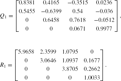
Example 9.5. Find the QR factorization of matrix A below:

Solution. Let Q = A = [u1 u2 u3 u4].
For i = 1,

For i = 2,

For i = 3,

For i = 4,
Therefore,

We obtain the factorization,

QR factorization is applied to find all the eigenvalues of a symmetrix matrix and their corresponding eigenvectors by factorizing the matrix as A = QR and by reversing the resulting factorization through a series of iterations until all the errors from the eigenvalues are smaller than a tolerated value ε. The error is computed as [λk+1 − λk], where k is the iteration number. The iterations are shown as

Convergence to the solution is said to be achieved once all the errors are less than the tolerated value ε. The eigenvalues of A appear along the diagonal of final value of Ak+1, whereas the columns of Sk are their corresponding orthonormal eigenvectors basis, listed in the same order as eigenvalues.
Algorithm 9.5 summarizes the QR algorithm for finding the eigenvalues of a symmetric matrix A. The algorithm is further illustrated in Example 9.6.
Example 9.6. Find all the eigenvalues and their corresponding eigenvectors of a symmetric matrix given by

Solution. Iteration 0:
Factorizing matrix A = Q0 R0, we have (from Example 9.5)

Reverse multiply these matrices to produce

Iteration 1:
Factorize A1 = Q1 R1 to produce
Reverse multiply Q1 and R1 to produce A2,

Continue the steps until iteration 13, where the error is less than ε, to produce

We obtain all the eigenvalues and eigenvectors of matrix A from A14 and S13, respectively, as follows:


The eigenvalue problem is illustrated in a project called Code9. The project displays the power and the shifted power methods for finding the most dominant and least dominant eigenvalues of a given nonsymmetric matrix, respectively. For the case of a symmetric matrix, the program applies the Householder transformation and QR method automatically to compute all the eigenvalues.
Figure 9.1 shows an output from Code9. The figure shows the complete results for finding the most dominant and least dominant eigenvalues and their corresponding eigenvectors of the following matrix:

Input for the matrix is provided in the form of edit boxes. The results from the power series methods are displayed in two list view tables, the most dominant in the left and the least dominant in the right. The two tables display the mk and vk values for k = 0, 1, ..., Stop, where Stop is the stopping number of the iterations that complies with the stopping criteria, given as [mk+1 − mk] < ε. For the case of a symmetric matrix, the QR method displays the eigenvalues and their corresponding eigenvectors separately in two list view tables.
The maximum size of the matrix allowed in this interface is 8 × 8. The user has the option of selecting the matrix size by filling in the values starting from the top left-hand corner of the edit boxes. The actual size of the matrix is determined from the diagonal elements. An empty entry for the diagonal element ai,i indicates the size of matrixis (i − 1) × (i − 1). Therefore, the program is flexible in the sense that it allows the user to determine the size of the matrix freely by entering values in the edit boxes.
Figure 9.2 shows a schematic drawing of the computational steps in Code9. The progress in the runtime is monitored through fStatus whose initial value is 0. This value changes to 1 when either the power method or the QR method has been successfully applied to solve the given problem. Edit boxes for the input are created in the constructor function, whereas their values are read in the OnButton() as soon as the Compute button is left-clicked.

The OnButton() performs a simple test to determine whether the input matrix is symmetric. If the matrix is symmetric, QRMtd() is called to execute the QR method. Otherwise, the processing is passed to PowerMtd(), which refers to the power method. A success in either method changes fStatus value to 1. The full eigenvalues and eigenvectors are then displayed in the list view tables through QRTable() for the QR method and PowerTable() for the power method.
Code9 consists of two files, Code9.h and Code9.cpp. A single class called CCode9 is used, and this class is derived from CFrameWnd. The main window from this class consists of two list view tables, 64 edit boxes for representing the 8 × 8 matrix, another edit box for the error stopping value ε, and a push button called Compute .
The elements in the iterations in the power and QR methods are represented by a structure called ITER, which are given by
typedef struct
{
      double lambda, v[M+1], error;
      double lambdaB, vB[M+1], errorB;
      double lambdaQR[M+1], vQR[M+1][M+1], errorQR[M+1];
} ITER;
ITER eigen[maxIter+1];
A maximum number of iterations allowed is a macro called maxIter. In the most dominant eigenvalue problem, an array called eigen stores the values of mk and vk for matrix A, for k = 0, 1, ..., Stop. Here, mk is represented by lambda and vk by the array v. In the least dominant eigenvalue problem, mk and vk of the matrix B are represented by lambdaB and vB, respectively. The errors in the iterations are error for the A matrix and errorB for the B matrix. For the QR method, lambdaQR and vQR are the eigenvalues and their corresponding eigenvectors, respectively. The error is errorQR.
The elements for the input boxes are represented by a structure called INPUT. The boxes form matrix A whose elements consist of the array input. The elements in the array are the edit boxes (ed), their home coordinates (hm), and their contents (item).
typedef struct
{
      CPoint hm;
      CString item;
      CEdit ed;
} INPUT;
INPUT input[nInputItems+1][M+1];
Table 9.3. Member functions in CCode6
Description | |
|---|---|
| Constructor. |
| Destructor. |
The power method for finding the most dominant eigenvalue and its corresponding eigenvector. | |
Computes all the eigenvalues and eigenvectors of a symmetrix matrix using the Householder transformation and QR method. | |
Creates a list view table to display the results. | |
Displays all the eigenvalues and their corresponding eigenvectors in two separate list view tables. | |
| Responds to ON BN CLICKED, which reads the input matrix from the user and calls the respective method to produce its solution. |
Displays and updates the output in the main window. |
Table 9.3 lists the functions in CCode9. The key function in this class is PowerMtd(), which computes the most dominant and least dominant eigenvalues of the input matrix A and its corresponding eigenvectors. PowerTable() displays the detail results from the iterations in two list view tables, one for the most dominant eigenvalue and another for the least dominant eigenvalue.
Table 9.4 lists the main variables and objects in CCode9. The progress in execution is marked using fStatus, where, fStatus=0 indicates the stage before the power method is applied, and fStatus=1 indicates the power method has been successfully applied. The maximum matrix size shown is M, whereas its actual size is m. The number of iterations performed before convergence in matrix A is indicated by Stop1, whereas that in matrix B is indicated by Stop2.
There are two events, an update in the main window and the push button click, and they are handled by OnPaint() and OnButton(), respectively.
BEGIN MESSAGE MAP(C Code9, CFrameWnd)
    ON WM PAINT()
    ON BN CLICKED(IDC BUTTON,  OnButton)
END MESSAGE MAP()
The OnButton() responds to the push button click. There are three local arrays in the function: A, B, and I.A is the original matrix whose most dominant eigenvalue is the first subject in the problem. B is A − λI, and its most dominant eigenvalue contributes to finding the least dominant eigenvalue for A.I is the identity matrix, which is needed in computing B. The function is given, as follows:
void CCode9::OnButton()
{
      int i,  j,  k;
      double **A, **B, **I;
A=new double *[M+1];
B=new double *[M+1];
I=new double *[M+1];
for (i=1;i<=M;i++)
{
A[i]=new double [M+1];
B[i]=new double [M+1];
I[i]=new double [M+1];
}
for (i=1;i<=M;i++)
      for (j=1;j<=M;j++)
input[i][j].ed.GetWindowText
                (input[i][j].item);
input[nInputItems][1].ed.GetWindowText
     (input[nInputItems][1].item);

// determine the actual size of matrix
for (i=1;i<=M;i++)
      if (input[i][i].item=="")
      {
            m=i-1; break;
}// read the contents of A
for (i=1;i<=m;i++)
      for (j=1;j<=m;j++)
      {
            I[i][j]=0;
            if (i==j)
                  I[i][j]=1;
            A[i][j]=atof(input[i][j].item);
        }
// test for matrix symmetry
k=0;
for (i=1;i<=m;i++)
for (j=1;j<=m;j++)
if (A[i][j]==A[j][i])
k++;
fMenu=((k==m*m)?2:1);
if (fMenu==1)
{
PowerMtd(1, A);
PowerTable(1);
if (StopA!=−1)
{
for (i=1;i<=m;i++)
for (j=1;j<=m;j++)
B[i][j]=A[i][j]-eigen[StopA]
.lambda*I[i][j];
PowerMtd(2, B);
PowerTable(2);
}
}
if (fMenu==2)
{
QRMtd(A);
QRTable(1);
QRTable(2);
}
}Table 9.4. Main variables and objects in Code9
Variable/object | Type | Description |
|---|---|---|
|
| A flag whose values are |
|
| The method assigned, with |
|
| Actual size and maximum size of A matrix, respectively. |
| Maximum size of the A matrix. | |
|
| Number of iterations before convergence to the most dominant and least dominant eigenvalues, respectively. |
|
| ε or the stopping criteria for the iterations in the power method. |
|
| Number of input items in the selected method. |
|
| Maximum number of iterations allowed for the power method. |
|
| Id for the edit boxes. |
|
| Push button object called Compute. |
The OnButton() first reads the input values from A beginning with the top row, from left to right. The size of A is determined in this function by detecting the first null entry in its diagonal element. A null entry at ai,i implies the size of the matrix is (i − 1) × (i − 1), and this assigns m = i − 1. The code fragments for this task are
for (i=1;i<=M;i++)
for (j=1;j<=M;j++)input[i][j].ed.GetWindowText
(input[i][j].item);
input[nInputItems][1].ed.GetWindowText
(input[nInputItems][1].item);
// determine the actual size of matrix
for (i=1;i<=M;i++)
if (input[i][i].item=="")
{
m=i-1; break;
}Once the actual size of the matrix is known, the corresponding identity matrix can now be created. At the same time, the values for A are determined by converting their corresponding strings in the edit boxes, as follows:
for (i=1;i<=m;i++)
for (j=1;j<=m;j++)
{
I[i][j]=0;
if (i==j)
I[i][j]=1;
A[i][j]=atof(input[i][j].item);
}The OnButton() calls PowerMtd() twice for computing the most dominant eigenvalues and their corresponding eigenvectors in A and B. The results from the iterations are displayed in the list view tables through PowerTable().
if (fMenu==1)
{
      PowerMtd(1, A);
      PowerTable(1);
      if (StopA!=−1)
      {
            for (i=1;i<=m;i++)
                  for (j=1;j<=m;j++)
                        B[i][j]=A[i][j]-eigen[StopA].
                                 lambda*I[i][j];
            PowerMtd(2, B);
            PowerTable(2);
      }
}
In the case where matrix A is symmetric, the flag fMenu=2 becomes active to indicate the problem is passed to the QR method in its solution. The code fragments are as follows:
if (fMenu==2)
{
      QRMtd(A);
      QRTable(1);
      QRTable(2);
}PowerMtd() computes the most dominant eigenvalue λ1 and its corresponding eigenvectors v1. There are two arguments in PowerMtd(). The first argument is fPower, and its value identifies the matrix to compute: 1 for A and 2 for B. The second argument is matrix c, which obtains its values through data passing from either A or B. The full code listing for PowerMtd() is given below:
void CCode9::PowerMtd(int fPower, double **c)
{
      double u[M+1], w[M+1], lamb[maxIter+1], error[maxIter+1];
      int i, j, k;
      for (i=1;i<=m;i++)
      {
           w[i]=0;
           if (i==2)
                 w[i]=1;
           eigen[0].v[i]=w[i];
           eigen[0].vB[i]=w[i];
      }
      epsilon=atof(input[nInputItems][1].item);
      for (k=0;k<=maxIter;k++)
      {
            for (i=1;i<=m;i++)
            {
                 u[i]=0;
                 for (j=1;j<=m;j++)
                       u[i] += c[i][j]*w[j];
            }
            lamb[k]=u[1];
            for (i=1;i<=m;i++)
                  if (fabs(lamb[k])<=fabs(u[i]))
                  {
                       lamb[k]=u[i];
                       if (fPower==1)
                             eigen[k+1].lambda=lamb[k];
if (fPower==2)
eigen[k+1].lambdaB=lamb[k];
}
for (i=1;i<=m;i++)
{
w[i]=u[i]/lamb[k];
if (fPower==1)
eigen[k+1].v[i]=w[i];
if (fPower==2)
eigen[k+1].vB[i]=w[i];
}
if (k>0)
{
error[k]=lamb[k]-lamb[k-1];
if (fPower==1)
eigen[k].error=error[k];
if (fPower==2)
eigen[k].errorB=error[k];
if (fabs(error[k])<epsilon)
{
if (fPower==1)
{
StopA=k;
eigen[StopA].lambda=lamb[StopA];
fStatus=1;
Invalidate();
break;
}
if (fPower==2)
{
StopB=k;
eigen[StopB].lambdaB=lamb[StopB];
break;
}
}
else
{
if (k==maxIter && fPower==1)
StopA=−1;
if (k==maxIter && fPower==2)
StopB=−1;
}
}
}
}In PowerMtd(), the initial values consist of v0 = [0 1 0]T for both matrix A and B, and ε. The code is given by
for (i=1;i<=m;i++)
{
      w[i]=0;
      if (i==2)
            w[i]=1;
      eigen[0].v[i]=w[i];
      eigen[0].vB[i]=w[i];
}
epsilon=atof(input[nInputItems][1].item);
Convergence to the solution is obtained from the error tolerance given by [λk+1 − λk] < ε, and this condition is applied through fabs(error[k])<epsilon. The conditional test is performed at every iteration to determine whether the error complies with the given tolerance. The last iteration numbers before convergence, StopA for matrix A and StopB for matrix B, are stored in order to display the eigenvalues and eigenvectors in list view tables later. The code for this task is given by
error[k]=lamb[k]-lamb[k-1];
if (fPower==1)
      eigen[k].error=error[k];
if (fPower==2)
      eigen[k].errorB=error[k];
if (fabs(error[k])<epsilon)
{
      if (fPower==1)
      {
            StopA=k;
            eigen[StopA].lambda=lamb[StopA];
            fStatus=1;
            Invalidate();
            break;
     }
     if (fPower==2)
     {
           StopB=k;
           eigen[StopB].lambdaB=lamb[StopB];
           break;
     }
}
else
{
if (k==maxIter && fPower==1)
StopA=−1;
if (k==maxIter && fPower==2)
StopB=−1;
}The QR method is handled by QRMtd(). The function computes all the eigenvalues belonging to a symmetric matrix through a conditional check performed by OnButton(). The function is given by
void CCode9::QRMtd(double **c)
{
      int i, j, k, u, p;
      double a[maxIter+1][M+1][M+1], r[M+1][M+1];
      double q[M+1][M+1], s[M+1][M+1], w[M+1][M+1];
      double t[M+1], P[M+1][M+1], I[M+1][M+1], B[M+1][M+1];
      double Alpha, R, Sum;
      epsilon=atof(input[nInputItems][1].item);
      for (i=1;i<=m;i++)
            for (j=1;j<=m;j++)
            {
                  r[i][j]=0;
                  a[0][i][j]=c[i][j];
                  I[i][j]=0;
                  if (i==j)
                        I[i][j]=1;
            }

      //Householder's Method
      for (k=1;k<=m-2;k++)
      {
            Sum=0;
            for (i=k+1;i<=m;i++)
                  Sum+=pow(a[0][i][k], 2);
            if (a[0][k+1][k]<0)
                  Alpha=sqrt(Sum);
            else
                  Alpha=(−1)*sqrt(Sum);
            R=sqrt((pow(Alpha, 2)*1/2)-(Alpha*a[0][k+1][k]*1/2));
            for (i=1;i<=k;i++)
                  t[i]=0;
            t[k+1]=(a[0][k+1][k]-Alpha)/(2*R);
for (i=k+2;i<=m;i++)
t[i]=a[0][i][k]/(2*R);
for (i=1;i<=m;i++)
for (j=1;j<=m;j++)
P[i][j]=I[i][j]-(2*t[i]*t[j]);
for (i=1;i<=m;i++)
for (j=1;j<=m;j++)
{
Sum=0;
for (u=1;u<=m;u++)
Sum+=P[i][u]*a[0][u][j];
B[i][j]=Sum;
}
for (i=1;i<=m;i++)
for (j=1;j<=m;j++)
{
Sum=0;
for (u=1;u<=m;u++)
Sum += B[i][u]*P[u][j];
a[0][i][j]=Sum;
}
}
for (i=1;i<=m;i++)
for (j=1;j<=m;j++)
q[i][j]=a[0][i][j];
//QR algorithm
StopA=−1;
for (p=0;p<=maxIter;p++)
{
for (i=1;i<=m;i++)
for (j=i;j<=m;j++)
{
if (i==j)
{
Sum=0;
for (k=1;k<=m;k++)
Sum+=pow(q[k][i], 2);
r[i][j]=pow(Sum, 0.5);
for (k=1;k<=m;k++)
q[k][j]=(q[k][j]/r[i][j]);
}
if (i<j)
{
Sum=0;for (k=1;k<=m;k++)
Sum+=(q[k][i]*q[k][j]);
r[i][j]=Sum;
for (k=1;k<=m;k++)
q[k][j]=q[k][j]-(r[i][j]
*q[k][i]);
}
}
if (p==0)
for (i=1;i<=m;i++)
for (j=1;j<=m;j++)
{
s[i][j]=q[i][j];
eigen[p].vQR[i][j]=q[j][i];
}
else
{
for (i=1;i<=m;i++)
for (j=1;j<=m;j++)
{
Sum=0;
for (k=1;k<=m;k++)
Sum+=s[i][k]*q[k][j];
w[i][j]=Sum;
}
for (i=1;i<=m;i++)
for (j=1;j<=m;j++)
{
s[i][j]=w[i][j];
eigen[p].vQR[i][j]=w[j][i];
}
}
for (i=1;i<=m;i++)
for (j=1;j<=m;j++)
{
Sum=0;
for (k=1;k<=m;k++)
Sum+=r[i][k]*q[k][j];
a[p][i][j]=Sum;
q[i][j]=a[p][i][j];
eigen[p].lambdaQR[i]=a[p][i][i];
}
if (p>0)
{
j=0;for (i=1;i<=m;i++)
{
eigen[p].errorQR[i]=eigen[p].lambdaQR[i]
-eigen[p-1].lambdaQR[i];
if (fabs(eigen[p].errorQR[i])<epsilon)
j++;
}
if (j==m)
{
fStatus=1;
Invalidate();
StopA=p;
break;
}
}
}
}QRMtd() consists of two major steps. First, the symmetric matrix is converted into a symmetric tridiagonal matrix through the Householder transformation. This is achieved through
//Householder's Method
for (k=1;k<=m-2;k++)
{
      Sum=0;
      for (i=k+1;i<=m;i++)
            Sum+=pow(a[0][i][k], 2);
      if (a[0][k+1][k]<0)
            Alpha=sqrt(Sum);
      else
            Alpha=(−1)*sqrt(Sum);
      R=sqrt((pow(Alpha, 2)*1/2)-(Alpha*a[0][k+1][k]*1/2));
      for (i=1;i<=k;i++)
            t[i]=0;
      t[k+1]=(a[0][k+1][k]-Alpha)/(2*R);
      for (i=k+2;i<=m;i++)
            t[i]=a[0][i][k]/(2*R);
      for (i=1;i<=m;i++)
            for (j=1;j<=m;j++)
                  P[i][j]=I[i][j]-(2*t[i]*t[j]);
      for (i=1;i<=m;i++)
            for (j=1;j<=m;j++)
            {
                  Sum=0;
for (u=1;u<=m;u++)
Sum+=P[i][u]*a[0][u][j];
B[i][j]=Sum;
}
for (i=1;i<=m;i++)
for (j=1;j<=m;j++)
{
Sum=0;
for (u=1;u<=m;u++)
Sum += B[i][u]*P[u][j];
a[0][i][j]=Sum;
}
}
for (i=1;i<=m;i++)
for (j=1;j<=m;j++)
q[i][j]=a[0][i][j];The second step consists of the application of the QR method in determining the eigenvalues and their corresponding eigenvectors. Iterations are performed using p until convergence, which is indicated by the integer variable, StopA. With the convergence, the flag status value is changed to fStatus=1, which means the method has been successfully applied. The eigenvalues are the last values of eigen[p].lambdaQR[i], whereas their eigenvectors are eigen[p].vQR[i]. The code fragments are given by
//QR algorithm
StopA=−1;
for (p=0;p<=maxIter;p++)
{
      for (i=1;i<=m;i++)
            for (j=i;j<=m;j++)
            {
                  if (i==j)
                  {
                        Sum=0;
                        for (k=1;k<=m;k++)
                              Sum+=pow(q[k][i], 2);
                        r[i][j]=pow(Sum, 0.5);
                        for (k=1;k<=m;k++)
                              q[k][j]=(q[k][j]/r[i][j]);
                  }
                  if (i<j)
                  {
                       Sum=0;
                       for (k=1;k<=m;k++)
Sum+=(q[k][i]*q[k][j]);
r[i][j]=Sum;
for (k=1;k<=m;k++)
q[k][j]=q[k][j]-(r[i][j]*q[k][i]);
}
}
if (p==0)
for (i=1;i<=m;i++)
for (j=1;j<=m;j++)
{
s[i][j]=q[i][j];
eigen[p].vQR[i][j]=q[j][i];
}
else
{
for (i=1;i<=m;i++)
for (j=1;j<=m;j++)
{
Sum=0;
for (k=1;k<=m;k++)
Sum+=s[i][k]*q[k][j];
w[i][j]=Sum;
}
for (i=1;i<=m;i++)
for (j=1;j<=m;j++)
{
s[i][j]=w[i][j];
eigen[p].vQR[i][j]=w[j][i];
}
}
for (i=1;i<=m;i++)
for (j=1;j<=m;j++)
{
Sum=0;
for (k=1;k<=m;k++)
Sum+=r[i][k]*q[k][j];
a[p][i][j]=Sum;
q[i][j]=a[p][i][j];
eigen[p].lambdaQR[i]=a[p][i][i];
}
if (p>0)
{
j=0;
for (i=1;i<=m;i++)
{eigen[p].errorQR[i]=eigen[p].lambdaQR[i]
-eigen[p-1].lambdaQR[i];
if (fabs(eigen[p].errorQR[i])<epsilon)
j++;
}
if (j==m)
{
fStatus=1;
Invalidate();
StopA=p;
break;
}
}Output in Code9 is produced in the form list view tables, which shows the results from every iteration. Two functions are created, PowerTable() for the results from power and shifted power methods and QRTable() for the QR method. The two functions are given as follows:
void CCode9::PowerTable(int c)
{
      int Stop, i, j, k;
      CString str;
      CRect rcTable[3];
      rcTable[c]=CRect(table[c].hm.x, table[c].hm.y, table[c].hm.x
                 +370, table[c].hm.y+290);
      table[c].list.DestroyWindow();
      table[c].list.Create(WS_VISIBLE | WS_CHILD | WS_DLGFRAME
            | LVS_REPORT | LVS_NOSORTHEADER, rcTable[c], this,
            idc++);
      table[c].list.InsertColumn(0, "i", LVCFMT_CENTER, 25);
      table[c].list.InsertColumn(1, ((c==1)?"lambda hi"
            :"lambda lo"), LVCFMT_CENTER, 70);
      for (i=2;i<=m+1;i++)
      {
            str.Format("v[%d]", i-1);
            table[c].list.InsertColumn(i, str, LVCFMT_CENTER, 70);
      }
      table[c].list.InsertColumn(m+2, "error", LVCFMT_CENTER, 70);
      Stop=((c==1)?StopA:StopB);
      for (k=0;k<=Stop;k++)
      {
            str.Format("%d", k);
table[c].list.InsertItem(k, str, 0);
if (k<0)
{
str.Format("%lf", ((c==1)?eigen[k].lambda
:eigen[k].lambdaB+eigen[StopA].lambda));
table[c].list.SetItemText(k, 1, str);
str.Format("%lf", ((c==1)?eigen[k].error:
eigen[k].errorB));
table[c].list.SetItemText(k, m+2, str);
}
for (j=1;j<=m;j++)
{
str.Format("%lf", ((c==1)?eigen[k].v[j]:
eigen[k].vB[j]));
table[c].list.SetItemText(k, j+1, str);
}
}
}
void CCode9::QRTable(int c)
{
int Stop, i, j, k, p;
CString str;
CRect rcTable[4];
rcTable[c]=CRect(table[c].hm.x, table[c].hm.y, table[c].hm.x
+370, table[c].hm.y+290);
table[c].list.DestroyWindow();
table[c].list.Create(WS_VISIBLE | WS_CHILD | WS_DLGFRAME
| LVS_REPORT | LVS_NOSORTHEADER, rcTable[c], this,
idc++);
table[c].list.InsertColumn(0, "i", LVCFMT_CENTER, 25);
if (c==1)
for (i=1;i<=m;i++)
{
str.Format("lambda[%d]", i);
table[c].list.InsertColumn(i, str,
LVCFMT_CENTER, 70);
str.Format("error[%d]", i);
table[c].list.InsertColumn(m+i, str,
LVCFMT_CENTER, 70);
}
if (c==2)
{
k=0;
for (i=1;i<=m;i++)for(j=1;j<=m;j++)
{
str.Format("v[%d][%d]", i, j);
table[c].list.InsertColumn
(i+k, str, LVCFMT_CENTER, 70);
k++;
}
}
Stop=StopA;
for (k=0;k<=Stop;k++)
{
str.Format("%d", k);
table[c].list.InsertItem(k, str, 0);
if (k>0)
{
if (c==1)
for (i=1;i<=m;i++)
{
str.Format("%lf", eigen[k].
lambdaQR[i]);
table[c].list.SetItemText(k, i,
str);
str.Format("%lf", eigen[k].
errorQR[i]);
table[c].list.SetItemText(k, m+i,
str);
}
if (c==2)
{
p=0;
for (i=1;i<=m;i++)
{
for (j=1;j<=m;j++)
{
str.Format("%lf", eigen[k]
.vQR[i][j]);
table[c].list.SetItemText
(k, j+p, str);
}
p += m;
}
}
}
}
}The chapter discusses the problem of finding eigenvalues of a given matrix. The power method has been applied in finding the most dominant eigenvalue, whereas its derivative called the shifted power method continues the step in determining the least dominant eigenvalue. Both methods also produce the corresponding eigenvectors for the computed eigenvalues through a series of iterations. In the case where the matrix is symmetric, a technique called the QR method is more practical as the method produces all the eigenvalues and their corresponding eigenvectors. The power, shifted power, and QR methods are illustrated in a project called Code9.
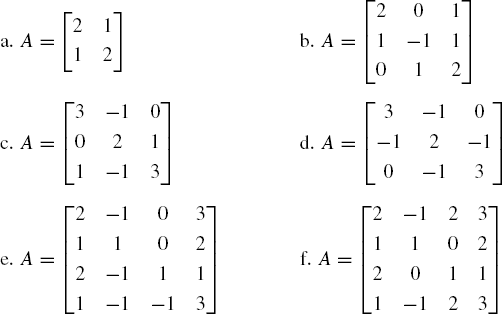
Find the most dominant and least dominant eigenvalues and their corresponding eigenvectors of the following matrices using the power and shifted power methods, with error tolerance of ε =0.05:
Check the results by running
Code9.Find all the eigenvalues and their corresponding eigenvectors of the following matrices using the QR method:
Check the results by running
Code9.

Modify
Code9by adding a new list view table to show the iterated values of the QR method.Modify
Code9by adding the file read and save options. Data to be read are in matrix A, which can have a size from 2 × 2 to 8 × 8, whereas for storage are the eigenvalues and eigenvectors.Modify
Code9by incorporating a method for detecting the singularity of the input matrix. A singular matrix A is one where |A| = 0, and this type of matrix does not have an inverse.