
Hour 5. Dates, Times, and Factors
What You’ll Learn in This Hour:
![]() How to create a date object
How to create a date object
![]() How to create a time object
How to create a time object
![]() How to manipulate date and time objects
How to manipulate date and time objects
![]() What a factor is and how to create one
What a factor is and how to create one
![]() How to manipulate factors
How to manipulate factors
In Hour 3, “Single-Mode Data Structures,” and Hour 4, “Multi-Mode Data Structures,” you saw how to create the basic data objects in R, objects that allow us to store numeric, logical, and character data.
In this hour, you learn more about some of the special data types in R that enable you to work with dates and times and with categorical data.
Working with Dates and Times
In this section, we look at how to convert date and time data into a format that R will recognize and manipulate.
Creating Date Objects
We can create a date object in R using the function as.Date. With this function we can create a vector of dates we can index in the same way we did in Hour 3. Most often our dates will be in the format of a character string, which we will convert to a date using the format argument to specify the structure of the date in the character string. You can see all of this in the following example:
> myDates <- c("2015-06-21", "2015-09-11", "2015-12-31")
> myDates <- as.Date(myDates, format = "%Y-%m-%d")
> myDates
[1] "2015-06-21" "2015-09-11" "2015-12-31"
> myDates[2:3]
[1] "2015-09-11" "2015-12-31"
class(myDates)
[1] "Date"
As you can see, this creates a special Date type object. When this is printed to the screen, you will see it in the format year-month-day. This is the standard R date format. In actual fact, R has created an object that represents an integer number of days since January 1, 1970:
> as.numeric(myDates)
[1] 16607 16689 16800
Tip: Date Formats
In these examples we used the format argument to as.Date. This argument allows us to specify the initial format of our date string. For more details on the specification of the format argument, see the help file for the function strptime.
If we were to give a numeric value to the function as.Date, we would also need to specify the origin, or starting point, for the counting of days. For instance, if we were to pass dates that were generated by Microsoft Excel, which start counting from January 1, 1900, we would need to tell R that this is the origin or date from which the counting should start. Here’s an example:
> as.Date(42174, origin = "1900-01-01")
[1] "2015-06-21"
So what if our date is in a numeric format, such as 20150621? In this instance we first need to convert our date to a character string and then convert to a date as we did previously, using the format argument to specify the structure of the dates:
> myDates <- c(20150621, 20150911, 20151231)
> myDates <- as.character(myDates)
> myDates <- as.Date(myDates, format = "%Y%m%d")
> myDates
[1] "2015-06-21" "2015-09-11" "2015-12-31"
You will see very soon how you can manipulate and work with this type of object further.
Creating Objects That Include Times
When you have data that also includes times, you will need to work with a different class of object to incorporate the additional information. Here, we will use POSIXct and POSIXlt objects to store dates and times down to milliseconds. The two classes are very similar, though POSIXct objects are more suitable for storing data n data frames, whereas POSIXlt objects are a more human-readable format.
The functions that we use to create these objects are as.POSIXct and as.POSIXlt. They work in very much the same way as the as.Date function we used in the previous section, but we can now include hours, minutes and seconds. Both functions work in the same way, so here we will only look at as.POSIXct. Here is an example:
> myTimes <- c("2015-06-21 14:22:00", "2015-09-11 10:23:32", "2015-12-31 23:59:59")
> myTimes <- as.POSIXct(myTimes, format = "%Y-%m-%d %H:%M:%S")
> myTimes
[1] "2015-06-21 14:22:00 BST" "2015-09-11 10:23:32 BST" "2015-12-31 23:59:59 GMT"
> class(myTimes)
[1] "POSIXct" "POSIXt"
Note: Time Zones
You will have noticed that the preceding example has converted the dates and times into both British Summer Time and Greenwich Mean Time. The default for the POSIX functions is to use the locale of the machine you are working on and account for daylight savings time, but we can control the time zone used with the argument tz, for instance:
as.POSIXct(myTimes, format = "%Y-%m-%d %H:%M:%S", tz = "US/Pacific")
For more information on how to define time zones, take a look at the help pages for “timezones.”
As with dates, times are stored as an integer value, though in the instance of times it is the number of seconds starting from 00:00:00 January 1, 1970 UTC.
Manipulating Dates and Times
Once we have converted our dates and times to the appropriate R format, we can do things like
> myDates + 1
[1] "2015-06-22" "2015-09-12" "2016-01-01"
which makes use of the storage as numeric values to add a day (or second in the case of POSIX objects) to the time we provide. When it comes to adding other amounts of time, you might find the lubridate package, which we will see in the next section, useful.
A number of functions allow us to extract information such as weekdays, months, and quarters:
> weekdays(myDates)
[1] "Sunday" "Friday" "Thursday"
> months(myDates)
[1] "June" "September" "December"
> quarters(myDates)
[1] "Q2" "Q3" "Q4"
However, the more useful functions for working with dates and times are diff and difftime. These two functions both find the differences between given dates and times but work in a slightly different way. First of all, the diff function takes a vector of date-times and returns a vector of the difference between consecutive values. Here’s an example:
> diff(myDates)
Time differences in days
[1] 82 111
The function difftime, on the other hand, requires two separate date objects and finds the difference between the two. This is particularly useful if you want to find the difference between a series of dates and a specific date—for instance, the number of days from the start of the new year to the values in a given vector:
> difftime(myDates, as.Date("2015-07-04"))
Time differences in days
[1] -13 69 180
One useful feature of this function is that you can change the unit used for the difference returned, so you can see the difference in weeks, days, hours, minutes, or seconds:
> difftime(myDates, as.Date("2015-07-04"), units = "weeks")
Time differences in weeks
[1] -1.857143 9.857143 25.714286
Tip: Date Sequences
You might want to know that you can also create dates and times using a special version of the seq function. For instance, try the following:
seq (as.Date("2015-01-01"), as.Date("2015-12-01"), by = "week")
This will create a sequence of dates from January 1st to December 1st in weekly increments.
The lubridate Package
Instead of using the functions we have seen so far that are in the base R installation, we can use a number of additional packages for working with dates and times. In this section we look at the lubridate package, which has been designed to simplify the way in which you work with dates and times, making it easier to read them in to R and easier to manipulate, particularly when it comes to adding a unit of time. Because this package is not available in the standard R installation, you will first need to install and load it. See Hour 2, “The R Environment,” for a reminder on installing and loading an R package.
This package includes a number of useful functions, such as now, which gives the current date and time:
> now()
The equivalent to this in the base functionality of R would be Sys.time. You will notice functions in lubridate have been named in what is intended to be a more user-friendly manner. Before we look at some of the other useful functions in this package, let’s first look at converting our character strings or numeric values into date formats. There are three main functions in lubridate for converting to a date: ymd, mdy, and dmy. The one to use will depend on the order in which the year, month, and day are provided.
> myDates <- c("2015-06-21", "2015-09-11", "2015-12-31")
> myDates <- ymd(myDates)
> myDates
[1] "2015-06-21 UTC" "2015-09-11 UTC" "2015-12-31 UTC"
You will notice here that we simply provided the vector of dates; we did not need to provide the separator or any other formatting for the dates. Because the lubridate package is intended to make reading data easier, it will try to automatically determine the format based on the function we have called. In this example, it assumes the data is in the format year, month, day. In most instances this will be sufficient; however, in the case of mixed separators, it may not be able to determine the format and will return an appropriate warning to inform you of that fact.
You will also notice that the date is in the time zone UTC, or Universal time. As with the usual date function, we can change the time zone that is used when we import our data with the argument tz. Also, the useful functions force_tz and with_tz allow us to change the time zone after converting it.
When it comes to times, we continue to use the three functions from earlier, but now we add on “_hms,” or simply use the function hm or hms. Here is an example:
myTimes <- c("14:22:00", "10:23:32", "23:59:59")
myTimes <- hms(myTimes)
myTimes
[1] "14H 22M 0S" "10H 23M 32S" "23H 59M 59S"
These functions make it much easier to work with unconventional date-time data—for instance, when you only have the date and hour of an observation rather than data down to the second.
Further useful functions in this package include year, month, and day, which allow us to add a given amount of a specific period, for instance 2 seconds or 3 months, to a date-time:
newYearEve <- ymd_hms("2015-12-31 23:59:59")
newYearEve + seconds(2)
[1] "2016-01-01 00:00:01 UTC"
newYearEve + months(3)
[1] "2016-03-31 23:59:59 UTC"
newYearEve - years(1)
[1] "2014-12-31 23:59:59 UTC"
Working with Categorical Data
When we work with categorical data in R, we need to use a special data type called a factor. A factor is simply a categorical variable that is made up of levels and labels. In this section you will see how to convert a vector of categorical data into a factor and how to further manipulate these special objects. You will also see how to convert continuous data to a factor using the cut function.
Creating Factors
You can convert a vector of numeric values or character strings into a factor using the factor function. The default behavior of this function is to use the unique values of the vector as the levels and labels for the factor in alphanumeric order. As an example, consider Listing 5.1.
1: > x <- c("B", "B", "C", "A", "A", "A", "B", "C", "C")
2: > x
3: [1] "B" "B" "C" "A" "A" "A" "B" "C" "C"
4: > mode(x)
5: [1] "character"
6: > class(x)
7: [1] "character"
8: >
9: > y <- factor(x)
10: > y
11: [1] B B C A A A B C C
12: Levels: A B C
13: > mode(y)
14: [1] "numeric"
15: > class(y)
16: [1] "factor"
As you can see in line 9, you can very simply create a factor from a vector of character strings. You will notice in lines 11 and 12 that the output is printed differently when it is converted to a factor, displaying not only the vector but the levels of the factor. There are a few things to take note of in the factor and the mode of the object itself.
Let’s first consider the mode, or the way in which a factor is stored. Notice on lines 13 and 14 that the mode of the factor is numeric. A factor in R is actually stored as integer values that match up to the levels. In this example, any elements with the label “A” are in fact stored as 1, “B” stored as 2, and “C” as 3. In general, this will not impact the way in which you work with a factor but is worth noting.
Caution: Numeric Factors
When working with factors that have numeric levels, be aware that although the labels will take the values of the individual levels, the factor will be stored as integer values starting from 1. If you want to convert your factor back to numeric values, you first need to convert to character strings and then to numeric values.
The second thing to consider is the way in which factor levels are determined. As mentioned earlier and shown in Listing 5.1, the default behavior is to order levels alphanumerically. In the preceding example, this was not a problem, but consider the following example, where we are using the sample function to randomly select 20 values from a vector (see Hour 6, “Common R Utility Functions,” for more details on this function):
> ratings <- c("Poor", "Average", "Good")
> myRatings <- sample(ratings, 20, replace = TRUE)
> factorRatings <- factor(myRatings)
> factorRatings
[1] Poor Average Good Poor Good Good Good Poor
[9] Average Poor Average Good Average Average Average Average
[17] Good Average Poor Good
Levels: Average Good Poor
You can see here that the levels of the factor have been ordered alphabetically, even though there is an ordering that is more sensible for this case. This will have an impact when you want the ordering of a factor to be correct (for instance, when creating graphics). You can control the order of the levels of your factors using the levels argument, as shown next:
> factorRatings <- factor(myRatings, levels = ratings)
> factorRatings
[1] Poor Average Good Poor Good Good Good Poor
[9] Average Poor Average Good Average Average Average Average
[17] Good Average Poor Good
Levels: Poor Average Good
Notice here that the levels are now ordered exactly as we have specified.
Tip: Reordering Factors
You can use the reorder function to change the order of the levels of a factor based on another vector. This is particularly useful when creating graphics.
Manipulating Factor Levels
After creating your factor, you can work with it as though it was any other character vector, for instance:
> y == "A"
[1] FALSE FALSE FALSE TRUE TRUE TRUE FALSE FALSE FALSE
However, if you want to change the levels of the factor, you can’t just use standard methods for indexing and changing vector elements. As an example, suppose we want to change the levels in the ratings example from “Poor” to “Negative”:
> factorRatings[factorRatings == "Poor"] <- "Negative"
Warning message:
In `[<-.factor`(`*tmp*`, factorRatings == "Poor", value = "Negative") :
invalid factor level, NA generated
This is because when we defined the levels of the factor, we restricted the values that the factor could take to these groups, so we can’t use the usual manipulation techniques because we have to change the set of allowed values for the factor. Instead, we will need to use the levels function:
> levels(factorRatings)
[1] "Poor" "Average" "Good"
> levels(factorRatings) <- c("Negative", "Average", "Positive")
> factorRatings
[1] Negative Average Positive Negative Positive Positive Positive
[8] Negative Average Negative Average Positive Average Average
[15] Average Average Positive Average Negative Positive
Levels: Negative Average Positive
Caution: Missing Values in a Factor
If you have introduced missing values into a factor, you will need to re-create the factor or replace the missing values with the previous value that they took, otherwise you will retain missing values in your factor.
Here, we have only used the levels function to change the names of existing levels to unique equivalent levels, but we can also use this function to reduce the set of levels. Suppose that we were only interested in which elements were “Negative” and we were not interested in the distinction between “Average” and “Positive”. We might want to combine these elements as one level of the factor:
> levels(factorRatings) <- c("Negative", "Other", "Other")
> factorRatings
[1] Negative Other Other Negative Other Other Other Negative
[9] Other Negative Other Other Other Other Other Other
[17] Other Other Negative Other
Levels: Negative Other
Creating Factors from Continuous Data
So far you have seen how to create a factor from data that is already categorical, but what about if you want to use a continuous variable as the basis for a factor? In this case, you can use the cut function. The cut function has a number of arguments that can help you control exactly how the categories are formed. See Table 5.1 for a list of the main arguments.
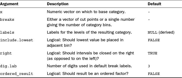
The simplest way you can create a factor is by providing the data and the breaks argument. Therefore, if you wanted to create three groups, you simply give breaks = 3, like so:
> ages <- c(19, 38, 33, 25, 21, 27, 27, 24, 25, 32)
> cut(ages, breaks = 3)
[1] (19,25.3] (31.7,38] (31.7,38] (19,25.3] (19,25.3] (25.3,31.7]
[7] (25.3,31.7] (19,25.3] (19,25.3] (31.7,38]
Levels: (19,25.3] (25.3,31.7] (31.7,38]
You can see in this example that the data has been split into three equally spaced levels. The levels are based on the range of the data rather than the number of values in each level. The levels here take the names of the ranges. You can have much more control over the ranges by instead specifying the lower and upper limits of each of the levels:
> cut(ages, breaks = c(18, 25, 30, Inf))
[1] (18,25] (30,Inf] (30,Inf] (18,25] (18,25] (25,30] (25,30] (18,25] (18,25]
[10] (30,Inf]
Levels: (18,25] (25,30] (30,Inf]
When you do this, you need to keep in mind that if the whole range of your data is not covered by the break points, you will introduce missing values, hence the use of Inf at the upper end. The arguments include.lowest and right let you control exactly where the group break points fall. Finally, you can control the labels that are given to the levels using the labels argument:
> cut(data, breaks = c(18, 25, 30, Inf), labels = c("18-25", "25-30", "30+"))
[1] 18-25 30+ 30+ 18-25 18-25 25-30 25-30 18-25 18-25 30+
Levels: 18-25 25-30 30+
As you can see, you can easily convert your continuous data to categories. You can see from Table 5.1 that there are more arguments that let you control the creation of the factor even further, including whether the groups are closed on the right or left (it defaults to left). We will use factors more when we manipulate data and create graphics, in particular when we use the package ggplot2 in Hour 14, “The ggplot2 Package for Graphics.”
Summary
In this hour we looked at some additional data types that allow us to work with dates and times and categorical data. You learned how to convert both numeric and character values into date and/or time objects and then how to manipulate these objects using the base functionality in R. You were also introduced to a useful package that can make these manipulations much simpler. Finally, you saw how R manages categorical data, how you can convert your data into this format, and how you can use continuous data to create your own categorical data. In the next hour, we look at some of the functions that we can use for working with the standard data types.
Q&A
Q. I have tried to convert my data to a Date object but it’s just returned a series of NA’s. Why doesn’t it recognize my data?
A. If you find you have been returned a series of NA’s after converting to a date or time, it is most likely because you have specified the wrong format in the format argument. Take a look at the help file for strptime for a full list of format codes, and don’t forget to include any spaces, dashes, or slashes in your dates.
Q. Why do I need to bother converting my data to a factor?
A. For general data-manipulation tasks, you will find that it makes very little difference whether your data is a factor or not. It will only be if you want to rename elements that you see a difference in behavior. Converting to a factor type is important when it comes to producing graphics and modeling your data. When you’re modeling, if your data is really categorical and you treat it as continuous, you will see a significantly different result. You will also find that if your data is large, then storing it as a factor is more efficient, as it will only store the unique values rather than repeating them a potential large number of times.
Workshop
The workshop contains quiz questions and exercises to help you solidify your understanding of the material covered. Try to answer all questions before looking at the “Answers” section that follows.
Quiz
1. What date does R use as the origin for counting dates and times?
2. What is the default time zone for creating POSIX objects?
3. What is a factor?
4. How are the levels of a factor determined?
5. If you were to use the function cut with the argument "breaks = 3", how would the levels be determined?
A. The data would be split into three equally sized groups based on the number of elements.
B. The range of the data would be split equally into three.
Answers
1. The origin for dates and times in R is January 1, 1970, 00:00:00 UTC.
2. The default time zone is the locale on your operating system. You can change the time zone using the tz argument. This is particularly useful if you are working with people across time zones and want to ensure the correct time zone for the data is used.
3. A factor is the way of storing categorical data in R.
4. If you choose not to give the appropriate levels using the levels argument, they will be the alphanumerically ordered unique elements of the data.
5. The answer is B. The range of the data is split equally to create three groups. This may mean, however, that the groups are of uneven size or the break points occur at locations that are not sensible for the data.
Activities
1. Create a vector of character strings that contains today’s date as well as the date of your next birthday and New Year’s Eve. Convert this character vector to a Date object.
2. Use the vector of dates to work out what day of the week your next birthday and New Year’s Eve occur on.
3. How many days are there from now until your next birthday?
4. Using the weather data we created in Hour 4, convert the Day column to a factor, ensuring that all possible days of the week can be used as levels and they are in the correct order, starting with Monday.
5. Change the levels of the Day factor column to be “Weekend” and “Weekday.”
6. Using the cut function, create a new column in the data, TempFactor, that takes the value “low” for temperatures less than 25, “medium” for temperatures from 25 to 30, and “high” for temperatures including and above 30 where all temperatures are in degrees Celsius.