
Hour 17. Common R Models
What You’ll Learn in This Hour:
![]() How to fit GLM Models
How to fit GLM Models
![]() How to fit Nonlinear Models
How to fit Nonlinear Models
![]() How to fit Survival Models
How to fit Survival Models
![]() How to fit Time Series Models
How to fit Time Series Models
In Hour 16, “Introduction to R Models and Object Orientation,” we explored the ways in which we can fit and assess statistical models in R. To achieve this, we used a simple linear modeling approach using the lm function. However, as mentioned, R has the most rich analytic feature set in any technology today. In this hour, we’ll extend the ideas of the previous hour to other modeling approaches. Specifically, we’ll look at Generalized Linear Models, Nonlinear Models, Time Series Models, and Survival Models. We’ll finish this hour by looking at other modeling approaches provided by R, and see where to access further information on these model types.
Note: Theory versus Code
In this hour, we provide a high-level overview of the theory for each modeling approach and then show how the models can be implemented in R. Consequently, we will not spend too much time on the detailed theory, or on the assessment of model performance, beyond that which helps you understand how methods can be applied to model objects.
Generalized Linear Models
In Hour 16, we used the lm function to fit Linear Models to our data. The “linear” aspect, here, refers to the fitting of a dependent variable against a linear function of independent variables. Here’s an example:
Y = θ0 + θ1X1 + θ2X2 + ... + θNXN + ε
Here, our Dependent Variable (Y) is modeled against N Independent Variables (X1 to XN), with parameters (θ0 to θN) to be estimated by the model-fitting process. With the Linear Model, such as that fit by the lm function, we make a number of assumptions. In particular, we assume that the Dependent Variable (Y) is continuous and Normally distributed. Furthermore, we assume the errors (ε) are independent and identically distributed such that E(ε) = 0 and var (ε) = σ2. We also assume that the errors (ε) are Normally distributed with mean 0 and variance σ2 for the purposes of tests.
GLM Definition
The Linear Model, described here, can be considered a special case of the Generalized Linear Model (GLM) framework. The GLM approach allows us to fit models where
![]() The Dependent Variable may not be continuous and Normally distributed.
The Dependent Variable may not be continuous and Normally distributed.
![]() The variance of the Dependent Variable may depend on the mean.
The variance of the Dependent Variable may depend on the mean.
The GLM framework uses four elements to fit a model:
![]() A probability distribution from the exponential family
A probability distribution from the exponential family
![]() A “linear predictor” to be modeled
A “linear predictor” to be modeled
![]() A “link function” defining how the linear predictor is related to the Dependent Variable
A “link function” defining how the linear predictor is related to the Dependent Variable
![]() A “variance function” explaining how the variance depends on the mean
A “variance function” explaining how the variance depends on the mean
In the GLM framework, the Dependent Variable (Y) is assumed to be generated from a specific distribution from the exponential family, a large range of distributions. A number of common distributions are listed in Table 17.1.

The linear predictor is of the following form:
γ = θ0 + θ1X1 + θ2X2 + ... + θNXN
Here, the linear predictor (γ) is linearly related to N Independent Variables (X1 to XN), with parameters (θ0 to θN) to be estimated by the model-fitting process.
The link function (g) is of the format g(μ) = γ and specifies how the linear predictor (γ) is related to the mean of the Dependent Variable, E(Y) = μ.
The variance function (V) explains how the variance of the Dependent Variable var (Y), depends on its mean (μ), specified as var (Y) = ϕV(μ). The variance function is typically dictated by the selected probability distribution.
Fitting a GLM
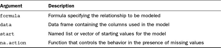
We can use the glm function to fit a Generalized Linear Model (GLM) in R. The key inputs to the glm function are listed in Table 17.2.

The formula, data, and na.action inputs are similar to the arguments seen with the lm function. Here, the formula describes the linear predictor we wish to model. The family input describes the link and variance function to be applied by the GLM framework. The family argument is typically specified as a character string or function. Some common examples are seen in Table 17.3, with further detail found in the ?family help file.

Fitting Gaussian Models
In Hour 16, we used the lm function to fit Linear Models to our data. This is, perhaps, the simplest case of the GLM framework, where
![]() The probability distribution is Gaussian.
The probability distribution is Gaussian.
![]() The link function is the identity function (because the linear predictor describes the Dependent Variance directly, without transformation).
The link function is the identity function (because the linear predictor describes the Dependent Variance directly, without transformation).
Thus, we can re-create a model from the previous chapter by instead using the glm function, as shown here:
> lmModel <- lm(mpg ~ wt * hp + factor(cyl), data = mtcars) # Model fit with lm
> lmModel
Call:
lm(formula = mpg ~ wt * hp + factor(cyl), data = mtcars)
Coefficients:
(Intercept) wt hp factor(cyl)6 factor(cyl)8 wt:hp
47.33733 -7.30634 -0.10333 -1.25907 -1.45434 0.02395
> glmModel <- glm(mpg ~ wt * hp + factor(cyl), data = mtcars) # Model fit with glm
> glmModel
Call: glm(formula = mpg ~ wt * hp + factor(cyl), data = mtcars)
Coefficients:
(Intercept) wt hp factor(cyl)6 factor(cyl)8 wt:hp
47.33733 -7.30634 -0.10333 -1.25907 -1.45434 0.02395
Degrees of Freedom: 31 Total (i.e. Null); 26 Residual
Null Deviance: 1126
Residual Deviance: 126.2 AIC: 148.7
We can see that the coefficients of both models match, as do the residuals produces from the models:
> all(signif(resid(lmModel), 10) == signif(resid(glmModel), 10))
[1] TRUE
Note: Default Family
Note here that “gaussian” is the default value of the family input, so we do not need to specify it here.
The glm Object
As with our earlier lm examples, the glm function returns an object that can be interrogated using a series of standard methods. A number of these standard methods can be seen in Table 17.4.

Detailed Summary
We can see a detailed model summary using the summary function, as shown here:
> summary(glmModel)
Call:
glm(formula = mpg ~ wt * hp + factor(cyl), data = mtcars)
Deviance Residuals:
Min 1Q Median 3Q Max
-3.5309 -1.6451 -0.4154 1.3838 4.4788
Coefficients:
Estimate Std. Error t value Pr(>|t|)
(Intercept) 47.337329 4.679790 10.115 1.67e-10 ***
wt -7.306337 1.675258 -4.361 0.000181 ***
hp -0.103331 0.031907 -3.238 0.003274 **
factor(cyl)6 -1.259073 1.489594 -0.845 0.405685
factor(cyl)8 -1.454339 2.063696 -0.705 0.487246
wt:hp 0.023951 0.008966 2.671 0.012865 *
---
Signif. codes: 0 '***' 0.001 '**' 0.01 '*' 0.05 '.' 0.1 ' ' 1
(Dispersion parameter for gaussian family taken to be 4.852119)
Null deviance: 1126.05 on 31 degrees of freedom
Residual deviance: 126.16 on 26 degrees of freedom
AIC: 148.71
Number of Fisher Scoring iterations: 2
Diagnostic Plots
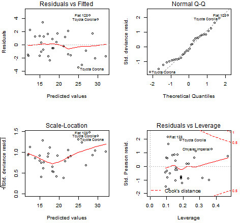
We can use the plot function to generate diagnostic plots of our model fit, as seen in Figure 17.1.
> par(mfrow = c(2, 2))
> plot(glmModel)
Functions such as coef, resid, and fitted can be used to extract model aspects, as seen in the following example. This includes the creation of a plot of residuals versus fitted values, as seen in Figure 17.2.
> coef(glmModel) # Model Coefficients
(Intercept) wt hp factor(cyl)6 factor(cyl)8 wt:hp
47.33732893 -7.30633653 -0.10333117 -1.25907265 -1.45433929 0.02395121
>
> res1 <- resid(glmModel) # Extract residuals
> fit1 <- fitted(glmModel) # Extract fitted values
> yRange <- c(-1, 1) * max(abs(res1)) # Calculate Y axis Range
> xRange <- range(fit1) # Calculate X axis Range
> xRange <- xRange + c(-1, 1) * diff(xRange)/5 # Extend X axis Range
>
> plot(fit1, res1, type = "n", # Empty plot with axes specified
+ ylim = yRange, xlim = xRange,
+ xlab = "Fitted Values", ylab = "Residuals",
+ main = "Residuals vs Fitted Values")
> text(fit1, res1, row.names(mtcars), cex=1.2) # Add text based on car names
> abline(h = 0, lty = 2) # Add horizontal reference line at 0

Logistic Regression
Logistic regression, or Logit Regression, is part of the GLM framework and can be implemented with the glm function. We use logistic regression to model the probability of some event occurring, based on a “dichotomous” Dependent Variable (that is, a variable with two levels specifying whether an event occurred). To achieve this, we model the log odds, so our link function (g) relates the Dependent Variable (Y) to the linear predictor (γ) via the logit function. Thus, ![]() . The Variance Function (V) is V(μ) = μ(1 – μ).
. The Variance Function (V) is V(μ) = μ(1 – μ).
Fitting a Logistic Regression
We fit a Logistic Regression using the glm function by specifying the binomial family. Our response variable must contain values 0 and 1 (or FALSE and TRUE). As a simple example, let’s model the am variable from the mtcars data based on wt. Here, we model the log-odds of the car having a manual transmission (am == 1) rather than an automatic transmission (am == 0), given the wt variable. The odds of interest can be calculated as the ratio of the probability of a manual transmission over that of an automatic one. Thus, log-odds are obtained through log transformation from the odds:
> lrModel <- glm(am ~ wt - 1, data = mtcars, family = binomial)
> summary(lrModel)
Call:
glm(formula = am ~ wt - 1, family = binomial, data = mtcars)
Deviance Residuals:
Min 1Q Median 3Q Max
-0.9397 -0.8525 -0.7549 1.4023 1.5541
Coefficients:
Estimate Std. Error z value Pr(>|z|)
wt -0.2388 0.1166 -2.049 0.0405 *
---
Signif. codes: 0 '***' 0.001 '**' 0.01 '*' 0.05 '.' 0.1 ' ' 1
(Dispersion parameter for binomial family taken to be 1)
Null deviance: 44.361 on 32 degrees of freedom
Residual deviance: 39.717 on 31 degrees of freedom
AIC: 41.717
Number of Fisher Scoring iterations: 4
Note: Removing the Intercept
We’ve removed the intercept in this example to better understand the resulting model coefficients.
Caution: Modeling Factor Levels
If the Dependent Variable specified is a two-level factor variable, R will model the probability of the second level occurring (so the first level is set as 0, and the second level as 1). If our Dependent Variable is a factor with levels “0” and “1,” this works as expected; however, care should be taken if you are using an unordered factor where the levels are defined alphabetically. For example, in the following, we would be modeling the probability of Y being “Low” instead of “High” because of the default alphabetic ordering of the factor levels:
> lrDf <- data.frame(Y = sample(c("Low", "High"), 10, T), X = rpois(10, 3))
> lrObj <- glm(Y ~ X, data = lrDf, family = binomial) # Logistic Model
> levels(lrDf$Y) # Ordering of levels
[1] "High" "Low"
Predictions from a Logistic Regression
When we use the predict function, we are (by default) predicting on the scale of the linear predictors (that is, we’re not directly predicting the responses). As such, the prediction function for our logistic example will return the log-odds of a car having a manual transmission. If we wish to see the predictions on the scale of the response, we set the type input to "response", which instead returns the probabilities.
> newDf <- data.frame(wt = 1:5)
> round(predict(lrModel, newDf), 4) # Log Odds
1 2 3 4 5
-0.2388 -0.4776 -0.7164 -0.9552 -1.1940
> round(predict(lrModel, newDf, type = "response"), 4) # Probability
1 2 3 4 5
0.4406 0.3828 0.3282 0.2778 0.2325
Coefficients from a Logistic Regression
As with predictions, the coefficients from a Logistic Regression are reported on the scale of the linear predictor. If we want to interpret the estimated effects as relative odds ratios, we simply exponentiate our coefficients as follows:
> round(coef(lrModel), 3) # Log-Odds
wt
-0.239
> round(exp(coef(lrModel)), 3) # Odds
wt
0.788
So, for every single unit increase in Weight, the odds of the car being manual (am = 1) are exected to decrease by a factor of 21% (e.g. Weight = 1, Odds = 0.79; Weight = 2, Odds = 0.79^2 = 0.62).
Tip: Confidence Intervals for Coefficients
The confint function will provide confidence intervals for coefficients in a glm (and lm) model. For example, we could provide estimates and confidence intervals for model coefficients on the log-odds scale using the following:
> cbind(coef(lrModel), confint(lrModel))
Waiting for profiling to be done...
[,1] [,2]
2.5 % -0.2388045 -0.48456168
97.5 % -0.2388045 -0.02093423
Poisson Regression
We can use Poisson regression, another example from the GLM framework, to model count data. This way, we can model the number of independent “events” to occur within a fixed “interval.” For a Poission regression, the link function (g) relates the Dependent Variable (Y) to the linear predictor (γ) via the log function, so g(μ) = log μ. The Variance Function (V) is V(μ) = μ.
Let’s fit a simple Poisson regression using glm. For this example, we’ll use the InsectSprays data frame, which has the counts of the number of insects based on the use of a variety of insecticides (see the ?InsectSprays help file for more information). Before we fit the model, let’s have a look at the data (seen here and in Figure 17.3):
> head(InsectSprays)
count spray
1 10 A
2 7 A
3 20 A
4 14 A
5 14 A
6 12 A
> plot(factor(InsectSprays$spray), InsectSprays$count,
+ xlab = "Insecticide", ylab = "Insect Count",
+ main = "Insect Count by Insecticide")

Let’s fit a simple Poisson model of count versus spray with no intercept term. We achieve this with glm by specifying poisson as the family input:
> prModel <- glm(count ~ factor(spray) - 1, data = InsectSprays, family = poisson)
> summary(prModel)
Call:
glm(formula = count ~ factor(spray) - 1, family = poisson, data = InsectSprays)
Deviance Residuals:
Min 1Q Median 3Q Max
-2.3852 -0.8876 -0.1482 0.6063 2.6922
Coefficients:
Estimate Std. Error z value Pr(>|z|)
factor(spray)A 2.67415 0.07581 35.274 < 2e-16 ***
factor(spray)B 2.73003 0.07372 37.032 < 2e-16 ***
factor(spray)C 0.73397 0.20000 3.670 0.000243 ***
factor(spray)D 1.59263 0.13019 12.233 < 2e-16 ***
factor(spray)E 1.25276 0.15430 8.119 4.71e-16 ***
factor(spray)F 2.81341 0.07071 39.788 < 2e-16 ***
---
Signif. codes: 0 '***' 0.001 '**' 0.01 '*' 0.05 '.' 0.1 ' ' 1
(Dispersion parameter for poisson family taken to be 1)
Null deviance: 2264.808 on 72 degrees of freedom
Residual deviance: 98.329 on 66 degrees of freedom
AIC: 376.59
Number of Fisher Scoring iterations: 5
Note: Including the Intercept
Note that, by suppressing the intercept, all levels of the factor variable are estimated (as opposed to the standard use of contrasts, where the first level would be set as the baseline). If, instead, we included an intercept term, then spray “A” would be set as the baseline and other coefficients would be interpreted in relation to this level:
> summary(glm(count ~ factor(spray), data = InsectSprays, family = poisson))$coef
Estimate Std. Error z value Pr(>|z|)
(Intercept) 2.67414865 0.0758098 35.2744434 1.448048e-272
factor(spray)B 0.05588046 0.1057445 0.5284477 5.971887e-01
factor(spray)C -1.94017947 0.2138857 -9.0711059 1.178151e-19
factor(spray)D -1.08151786 0.1506528 -7.1788745 7.028761e-13
factor(spray)E -1.42138568 0.1719205 -8.2676928 1.365763e-16
factor(spray)F 0.13926207 0.1036683 1.3433422 1.791612e-01
We can exponentiate the coefficients to see them on the scale of the response (that is, counts). Let’s see the exponentiated coefficients next to the confidence intervals:
> lc <- cbind(Est = coef(prModel), confint(prModel))
Waiting for profiling to be done...
> round(exp(lc), 2)
Est 2.5 % 97.5 %
factor(spray)A 14.50 12.45 16.76
factor(spray)B 15.33 13.22 17.66
factor(spray)C 2.08 1.37 3.01
factor(spray)D 4.92 3.77 6.28
factor(spray)E 3.50 2.55 4.67
factor(spray)F 16.67 14.46 19.08
GLM Extensions
So far we have looked at some Generalized Linear Model examples. Specifically, we have seen an example of a General Linear Model, a Logistic Regression, and a Poisson Regression. There are many related approaches and extensions that may be useful, including the following:
![]() We have bypassed the fitting of Analysis of Variance models, which can be achieved with the
We have bypassed the fitting of Analysis of Variance models, which can be achieved with the aov function (see the ?aov help file for details).
![]() There are many other distributions supported by
There are many other distributions supported by glm, which can be seen in the ?family help file.
![]() There are many extensions to the
There are many extensions to the glm function itself, such as the glm.nb function from the MASS package, which includes the estimation of the additional parameter “theta.”
![]() Extensions such as Generalized Estimating Equations (GEEs) allow for correlations between observations and are implemented in packages such as gee and geepack.
Extensions such as Generalized Estimating Equations (GEEs) allow for correlations between observations and are implemented in packages such as gee and geepack.
![]() Mixed models allow for random effects in the linear predictor and can be fit using packages such as lme4, nlme, and glmm.
Mixed models allow for random effects in the linear predictor and can be fit using packages such as lme4, nlme, and glmm.
![]() Generalized Additive Models (GAMs) allow the linear predictor to use smoothing functions applied to the Independent Variables. They are implemented in the gam package.
Generalized Additive Models (GAMs) allow the linear predictor to use smoothing functions applied to the Independent Variables. They are implemented in the gam package.
Nonlinear Models
The Generalized Linear Modeling approach allows us to fit a range of models where a Dependent Variable is related to a set of Independent Variables in a linear manner. However, R provides a range of functionality for fitting models where the function is a Nonlinear combination of parameters and depends on one or more Independent Variables.
Nonlinear Regression
The simplest form of Nonlinear model is a Nonlinear regression, which we can fit in R via least-squares estimation using the nls function. For Nonlinear regression,
Y = f(θ0, ..., M, X1,...,N) + ε
Here, our Dependent Variable (Y) is modeled against N Independent Variables (X1 to XN) and M parameters (θ0 to θM) to be estimated by the model-fitting process. We assume the errors (ε) are independent and identically distributed such that E(ε) = 0 and var(ε) = σ2. We also assume that the errors (ε) are Normally distributed with mean 0 and variance σ2 for the purposes of the tests.
Fitting a Nonlinear Regression
We can fit a Nonlinear model using least squares estimation with the nls function. The primary arguments accepted by nls can be seen in Table 17.5.
When we fit a Nonlinear model, it is common to define the relationship in terms of a function that accepts independent variables and parameters and returns a response.
As a very simple example, just to illustrate the use of nls, let’s fit our earlier linear model (of mpg vs wt). First, we’ll define a function we can use in our model fit and illustrate the use of the function with a two possible sets of input parameters (seen in Figure 17.4):
> linFun <- function(wt, a, b) a + b * wt
> plot(mtcars$wt, mtcars$mpg,
+ main = "Miles per Gallon versus Weight",
+ xlab = "Weight", ylab = "Miles per Gallon")
> lines(1:6, linFun(1:6, a = 40, b = -6), col = "red")
> lines(1:6, linFun(1:6, a = 35, b = -4.5), col = "blue")
> legend("topright", paste("Model", 1:2), fill = c("red", "blue"))
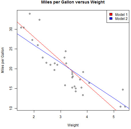
If we want to fit this as a Nonlinear(!) model, we use the nls function as follows:
> nlsMpg <- nls(mpg ~ linFun(wt, a, b), data = mtcars)
Warning message:
In nls(mpg ~ linFun(wt, a, b), data = mtcars) :
No starting values specified for some parameters.
Initializing 'a', 'b' to '1.'.
Consider specifying 'start' or using a selfStart model
Unfortunately, our model process fails because we have not provided starting values for the parameters (a and b). We can provide these as a named list or named vector of inputs. Based on the previous graph, let’s choose a = 40 and b = -5 as suitable starting parameters for our model:
> nlsMpg <- nls(mpg ~ linFun(wt, a, b), data = mtcars,
+ start = c(a = 40, b = -5))
> nlsMpg
Nonlinear regression model
model: mpg ~ linFun(wt, a, b)
data: mtcars
a b
37.285 -5.344
residual sum-of-squares: 278.3
Number of iterations to convergence: 1
Achieved convergence tolerance: 1.765e-09
As you can see, we have successfully fit our model and retrieved the parameters we would have achieved using a linear model (with the lm function):
> coef(nlsMpg) # Coefficients from the nls fit
a b
37.285126 -5.344472
> coef(lm(mpg ~ wt, data = mtcars)) # Coefficients from the lm fit
(Intercept) wt
37.285126 -5.344472
Let’s switch to using a more appropriate example.
Nonlinear Regression of the Puromycin Data
The Puromycin data frame in R contains data on the reaction velocity versus substrate concentration in an enzymatic reaction with Puromycin (an antibiotic). The data contains measurements involving untreated and treated cells. Let’s look at the data before we perform any model fitting, including a plot of the data in Figure 17.5:
> head(Puromycin) # A look at the data
conc rate state
1 0.02 76 treated
2 0.02 47 treated
3 0.06 97 treated
4 0.06 107 treated
5 0.11 123 treated
6 0.11 139 treated
> plot(Puromycin$conc, Puromycin$rate, pch = 21, cex = 1.5, # Plot the data
+ xlab = "Instantaneous reaction rates (counts/min/min)",
+ ylab = "Substrate Concentrations (ppm)",
+ main = "Instantaneous reaction rates vs Substrate Concentrations",
+ bg = ifelse(Puromycin$state == "treated", "red", "blue"))
> legend("bottomright", c("Treated", "Untreated"), fill = c("red", "blue"))

Let’s attempt to fit a Michaelis-Menten model to this data, which is one of the best-known models of enzyme kinetics. Given the preceding plot, we’ll fit separate models for “Treated” and “Untreated.” First, we’ll define the function and look at some possible starting values, overlaid on the previous plot. The output can be seen as Figure 17.6.
> micmen <- function(conc, Vm, K) Vm * conc / (K + conc) # Define function
> X <- seq(0, 1.1, length = 25) # Set of Concentrations
>
> lines(X, micmen(xConcs, 200, 0.1), col = "pink") # Treated: Vm = 200, K = 0.1
> lines(X, micmen(xConcs, 210, 0.03), col = "pink") # Treated: Vm = 210, K = 0.03
> lines(X, micmen(xConcs, 210, 0.05), col = "red") # Treated: Vm = 210, K = 0.05
>
> lines(X, micmen(xConcs, 150, 0.05), col = "lightblue") # Untreated: Vm = 150, K = 0.05
> lines(X, micmen(xConcs, 170, 0.1), col = "lightblue") # Untreated: Vm = 170, K = 0.1
> lines(X, micmen(xConcs, 165, 0.05), col = "blue") # Untreated: Vm = 165, V = 0.05

Based on this, let’s fit Nonlinear models to both the “Treated” and “Untreated” data:
> mmTreat <- nls(rate ~ micmen(conc, Vm, K), data = Puromycin,
+ start = c(Vm = 210, K = 0.05), subset = state == "treated")
> mmUntreat <- nls(rate ~ micmen(conc, Vm, K), data = Puromycin,
+ start = c(Vm = 165, K = 0.05), subset = state == "untreated")
> round(coef(mmTreat), 3) # Coefficients for Treated data
Vm K
212.684 0.064
> round(coef(mmUntreat), 3) # Coefficients for Untreated data
Vm K
160.280 0.048
Tip: Self-Starting Functions
In these examples, we need to specify starting values for our model fit. However, there are a number of “self-starting” functions in R that deduce starting values as part of the modeling process. These functions start with “SS” and can be listed using the following syntax:
> apropos("^SS")
[1] "SSasymp" "SSasympOff" "SSasympOrig" "SSbiexp"
[5] "SSD" "SSfol" "SSfpl" "SSgompertz"
[9] "SSlogis" "SSmicmen" "SSweibull"
Notice the SSmicmen function, which is a “self-starting” function that implements the Michaelis-Menten model. As such, we could simplify the preceding call as follows:
> nls(rate ~ SSmicmen(conc, Vm, K), data = Puromycin, subset = state == "treated")
Nonlinear regression model
model: rate ~ SSmicmen(conc, Vm, K)
data: Puromycin
Vm K
212.68371 0.06412
residual sum-of-squares: 1195
Number of iterations to convergence: 0
Achieved convergence tolerance: 1.93e-06
Making Predictions
We can use the predict function to make predictions from a Nonlinear model and then use the lines function to add the model lines to our plot. The result of this can be seen in Figure 17.7.
> plot(Puromycin$conc, Puromycin$rate, pch = 21, cex = 1.5,
+ xlab = "Instantaneous reaction rates (counts/min/min)",
+ ylab = "Substrate Concentrations (ppm)",
+ main = "Instantaneous reaction rates vs Substrate Concentrations",
+ bg = ifelse(Puromycin$state == "treated", "red", "blue"))
>
> predDf <- data.frame(conc = seq(0, 1.1, length = 25)) # Set of
Concentrations
> lines(predDf$conc, predict(mmTreat, predDf), col = "red") # Model for Treated
data
> lines(predDf$conc, predict(mmUntreat, predDf), col = "blue") # Model for
Untreated data
> legend("bottomright", c("Treated", "Untreated"), fill = c("red", "blue"))

Extended Model
We could extend our example to fit a single model that includes both the treated and untreated data. At the same time, we could add a new parameter to explain the difference in Vm between the two states. The outcome can be seen in Figure 17.8.
> # Add new parameter to out function (vTrt)
> micmen <- function(conc, state, Vm, K, vTrt) {
+ newVm <- Vm + vTrt * (state == "treated")
+ newVm * conc / (K + conc) # Define function
+ }
> mmPuro <- nls(rate ~ micmen(conc, state, Vm, K, vTrt), data = Puromycin,
+ start = c(Vm = 160, K = 0.05, vTrt = 50))
> summary(mmPuro)
Formula: rate ~ micmen(conc, state, Vm, K, vTrt)
Parameters:
Estimate Std. Error t value Pr(>|t|)
Vm 166.60396 5.80742 28.688 < 2e-16 ***
K 0.05797 0.00591 9.809 4.37e-09 ***
vTrt 42.02591 6.27214 6.700 1.61e-06 ***
---
Signif. codes: 0 '***' 0.001 '**' 0.01 '*' 0.05 '.' 0.1 ' ' 1
Residual standard error: 10.59 on 20 degrees of freedom
Number of iterations to convergence: 5
Achieved convergence tolerance: 9.239e-06
>
> plot(Puromycin$conc, Puromycin$rate, pch = 21, cex = 1.5,
+ xlab = "Instantaneous reaction rates (counts/min/min)",
+ ylab = "Substrate Concentrations (ppm)",
+ main = "Instantaneous reaction rates vs Substrate Concentrations",
+ bg = ifelse(Puromycin$state == "treated", "red", "blue"))
> xConc = seq(0, 1.1, length = 25) # Set of Concentrations
> trtPred <- data.frame(conc = xConc, state = "treated")
> untrtPred <- data.frame(conc = xConc, state = "untreated")
>
> lines(predDf$conc, predict(mmPuro, trtPred), col = "red") # Model for Treated
data
> lines(predDf$conc, predict(mmPuro, untrtPred), col = "blue") # Model for
Untreated data
> legend("bottomright", c("Treated", "Untreated"), fill = c("red", "blue"))

If we extract the coefficients from our model, we can see the highly significant vTrt variable:
> round(cbind(Est = coef(mmPuro), confint(mmPuro)), 3)
Waiting for profiling to be done...
Est 2.5% 97.5%
Vm 166.604 154.617 179.252
K 0.058 0.046 0.072
vTrt 42.026 28.957 55.199
Nonlinear Model Extensions
The previous section contained a very simple introduction to the Nonlinear model-fitting features of R. There are a number of extensions, including the following:
![]() The
The gnls function, which additionally allows for the correlated errors. For more information, see the ?gnls help file.
![]() The gnm package, which fits Generalized Nonlinear models (analogous to the
The gnm package, which fits Generalized Nonlinear models (analogous to the glm function for Nonlinear fits).
![]() The nlme package, which provides functionality for fitting Nonlinear Mixed Effects models.
The nlme package, which provides functionality for fitting Nonlinear Mixed Effects models.
Survival Analysis
Earlier in this hour, you saw how logistic regression can be used to model the probably of an event occurring. Survival analysis, instead, allows us to model the time until an event happens. For example, Survival analysis is used heavily in the field of medicine to understand the time until an event occurs, such as failure of an organ following transplant or time until death for someone with a terminal disease. We are interested in how a set of covariates may influence the time to event.
The ovarian Data Frame
Throughout this section we’ll use a data frame called ovarian, which contains data from a randomized trial comparing two treatments for ovarian cancer. This data frame can be found in the survival package:
> library(survival)
> head(ovarian)
futime fustat age resid.ds rx ecog.ps
1 59 1 72.3315 2 1 1
2 115 1 74.4932 2 1 1
3 156 1 66.4658 2 1 2
4 421 0 53.3644 2 2 1
5 431 1 50.3397 2 1 1
6 448 0 56.4301 1 1 2
The columns from the ovarian data frame are described in Table 17.6.

Censoring
When we are analyzing the time until an event occurs, a particular challenge is that the data may be “censored.” In this case, the event has not yet occurred, so we record the last times at which we know the events had not yet occurred and flag these observations. Consider if we wanted to understand the time an organ survives following a transplant. There are three possible outcomes:
![]() The organ is still functioning, so the failure of this organ has not yet occurred.
The organ is still functioning, so the failure of this organ has not yet occurred.
![]() The patient died as a result of something other than the organ failing.
The patient died as a result of something other than the organ failing.
![]() The organ failed, so the “event” has occurred.
The organ failed, so the “event” has occurred.
In the first two situations, the time is “censored” as we know the time until the “event” had not occurred, but cannot observe the time until the “event” itself.
In the case of our ovarian data frame, the time and “censor” flag are recorded in the futime and fustat variables.
> aggregate(ovarian$futime, list(State = ovarian$fustat),
+ function(x) c(Min = min(x), Median = median(x), Max = max(x)))
State x.Min x.Median x.Max
1 0 377.0 786.5 1227.0
2 1 59.0 359.0 638.0
Here, the censored times are those with State 0. We can create an object that combines these variables into a single object with the Surv function, as follows:
> ovSurv <- Surv(ovarian$futime, event = ovarian$fustat)
> ovSurv
[1] 59 115 156 421+ 431 448+ 464 475 477+ 563 638 744+ 769+ 770+
[15] 803+ 855+ 1040+ 1106+ 1129+ 1206+ 1227+ 268 329 353 365 377+
Note the + suffix for censored values (that is, observations where the event has not yet occurred).
Estimating the Survival Function
Much of Survival analysis is concerned with modeling and estimating the “Survival Function” (S), which provides the probability that an individual will survive a certain time (t). Formally,
S(t) = P(T > t) for times T ≥ 0
Consider the graphical representation of an example of a Survival Function shown in Figure 17.9.

Note that the probability of surviving past time t = 40 in Figure 17.9 is 39%. There are other characteristics of a Survival Function as t ranges from 0 to ∞, such as the following:
![]() The Survival Function is decreasing (or at least is non-increasing).
The Survival Function is decreasing (or at least is non-increasing).
![]() Typically, the probability of surviving past time 0 is 1, so S(0) = 1.
Typically, the probability of surviving past time 0 is 1, so S(0) = 1.
![]() The probability of surviving at time ∞ is 0, so S(∞) = 0.
The probability of surviving at time ∞ is 0, so S(∞) = 0.
We can estimate the Survival Function using either non-parametric or parametric approaches.
Kaplan-Meier Estimate
The “Kaplan-Meier” estimator (or “product limit” estimator) is the most popular non-parametric method statistic used to estimate the Survival Function. We can produce a Kaplan-Meier estimate in R using the survfit function. The first argument to the survfit function should be a formula with a survival object (such as the one we produced earlier) on its left hands side. To estimate a single Survival Function, we specify “1” on the right side, as follows:
> kmOv <- survfit(ovSurv ~ 1)
> kmOv
Call: survfit(formula = ovSurv ~ 1)
records n.max n.start events median 0.95LCL 0.95UCL
26 26 26 12 638 464 NA
The survfit function returns an object of class “survfit,” which has a few methods available. The summary method returns the estimated Survival Function along with confidence intervals:
> summary(kmOv)
Call: survfit(formula = ovSurv ~ 1)
time n.risk n.event survival std.err lower 95% CI upper 95% CI
59 26 1 0.962 0.0377 0.890 1.000
115 25 1 0.923 0.0523 0.826 1.000
156 24 1 0.885 0.0627 0.770 1.000
268 23 1 0.846 0.0708 0.718 0.997
329 22 1 0.808 0.0773 0.670 0.974
353 21 1 0.769 0.0826 0.623 0.949
365 20 1 0.731 0.0870 0.579 0.923
431 17 1 0.688 0.0919 0.529 0.894
464 15 1 0.642 0.0965 0.478 0.862
475 14 1 0.596 0.0999 0.429 0.828
563 12 1 0.546 0.1032 0.377 0.791
638 11 1 0.497 0.1051 0.328 0.752
The plot method allows us to produce a graph of the Kaplan-Meier estimate, seen in Figure 17.10.
> plot(kmOv, col = "blue",
+ main = "Kaplan-Meier Plot of Ovarian Data",
+ xlab = "Time (t)", ylab = "Survival Function S(t)")

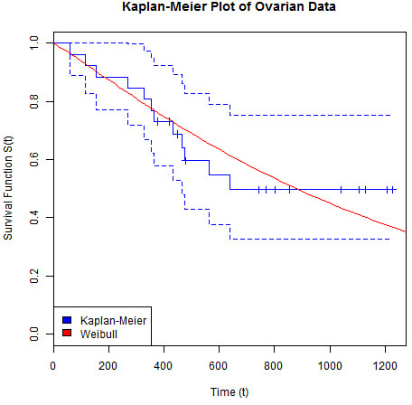
Parametric Methods
We can estimate the Survival Function using parametric methods with probability distributions such as Weibull, Exponential, and Log-Normal. In this case, we use maximum likelihood estimation to estimate the (unknown) parameters of the selected distribution. Let’s use the Weibull distribution to model the Survival, such that S(t) = exp (– α * tγ). We can fit a parametric survival model using the survreg function, which has a dist input for specifying the distribution:
> wbOv <- survreg(ovSurv ~ 1, dist = "weibull")
> summary(wbOv)
Call:
survreg(formula = ovSurv ~ 1, dist = "weibull")
Value Std. Error z p
(Intercept) 7.111 0.293 24.292 2.36e-130
Log(scale) -0.103 0.254 -0.405 6.86e-01
Scale= 0.902
Weibull distribution
Loglik(model)= -98 Loglik(intercept only)= -98
Number of Newton-Raphson Iterations: 5
n= 26
If we want to plot the line, there are two possible options:
![]() Manually transform the parameters into a Weibull curve
Manually transform the parameters into a Weibull curve
![]() Use the
Use the predict function
Let’s use the predict function, which allows us to produce a number of predictions from a “survfit” object. We can specify “quantile” predictions using type = "quantile", using the p argument to specify the quantiles for which to provide predictions. Because we have no covariates, we need to provide a “dummy” dataset for the newdata argument as follows:
> pct <- seq(.0,.99,by=.01) # Quantiles at which to predict
> dummyDf <- data.frame(1) # Dummy dataset
> predOv <- predict(wbOv, newdata = dummyDf, # Make Quantile predictions
+ type = "quantile", p = pct)
> head(predOv)
[1] 0.00000 19.28838 36.22041 52.46544 68.33554 83.97347
This returns a set of predicted time points for the specified quantiles. We can overlay these predictions onto our Kaplan-Meier plot, the output of which can be seen in Figure 17.11.
> plot(kmOv, col = "blue",
+ main = "Kaplan-Meier Plot of Ovarian Data",
+ xlab = "Time (t)", ylab = "Survival Function S(t)")
> lines(predOv, 1 - pct, col = "red")
> legend("bottomleft", c("Kaplan-Meier", "Weibull"), fill = c("blue", "red"))
Adding Covariates
We can easily add independent variables in the parametric model fit by specifying them on the right side of our formula. Let’s model survival against age using our ovarian data:
> wbOv2 <- survreg(ovSurv ~ age, dist = "weibull", data = ovarian)
> summary(wbOv2)
Call:
survreg(formula = ovSurv ~ age, data = ovarian, dist = "weibull")
Value Std. Error z p
(Intercept) 12.3970 1.4821 8.36 6.05e-17
age -0.0962 0.0237 -4.06 4.88e-05
Log(scale) -0.4919 0.2304 -2.14 3.27e-02
Scale= 0.611
Weibull distribution
Loglik(model)= -90 Loglik(intercept only)= -98
Chisq= 15.91 on 1 degrees of freedom, p= 6.7e-05
Number of Newton-Raphson Iterations: 5
n= 26
Let’s again use the predict function to create estimated Survival curves from different age groups. The output can be seen in Figure 17.12.
> ageDf <- data.frame(age = 10*4:6) # Set of ages for predictions
> theCols <- c("red", "blue", "green") # Colors to use
> predOv <- predict(wbOv2, newdata = ageDf, # Make Quantile predictions
+ type = "quantile", p = pct)
> matplot(t(predOv), 1-pct, xlim = c(0, 1200), # Matrix plot of predicted survival
+ type = "l", lty = 1, col = theCols,
+ main = "Parametric Estimation of Survival Curve by Age",
+ xlab = "Time (t)", ylab = "Survival Function S(t)")
> legend("bottomleft", paste("Age =", ageDf$age), fill = theCols)

Proportional Hazards
Proportional Hazards regression (or “Cox” regression) provides an excellent framework for modeling time to event data when we want to test many independent variables. In particular, Proportional Hazards regression provides a framework for understanding how differing levels of covariates increase the “risk” on a subject.
Proportional Hazards regression focuses on models of the “Hazard” Function (h), which can be considered as the probability of an event during an infinitesimally small period of time, and thus represents the “risk” of an event occurring at a specific point in time given that it hasn’t happened up to that point.
When we introduce Independent Variables into a Proportional Hazards regression, we can consider the Survival Model to have two components:
![]() An underlying baseline Hazard Function describing the “risk” over time at baseline levels of covariates
An underlying baseline Hazard Function describing the “risk” over time at baseline levels of covariates
![]() The effect parameters describing how the Hazard varies due to other (non-baseline) levels of covariates
The effect parameters describing how the Hazard varies due to other (non-baseline) levels of covariates
For a Proportional Hazards model to be suitable, the “Proportional Hazards condition” must hold, which states that covariates are related to the hazard in a multiplicative sense. We’ll check this assumption later.
To fit a Proportional Hazards model in R, we use the coxph function, and again we define the model to fit as a formula with a survival object on the left side:
> coxModel <- coxph(ovSurv ~ age + factor(rx), data = ovarian)
> summary(coxModel)
Call:
coxph(formula = ovSurv ~ age + factor(rx), data = ovarian)
n= 26, number of events= 12
coef exp(coef) se(coef) z Pr(>|z|)
age 0.14733 1.15873 0.04615 3.193 0.00141 **
factor(rx)2 -0.80397 0.44755 0.63205 -1.272 0.20337
---
Signif. codes: 0 '***' 0.001 '**' 0.01 '*' 0.05 '.' 0.1 ' ' 1
exp(coef) exp(-coef) lower .95 upper .95
age 1.1587 0.863 1.0585 1.268
factor(rx)2 0.4475 2.234 0.1297 1.545
Concordance= 0.798 (se = 0.091 )
Rsquare= 0.457 (max possible= 0.932 )
Likelihood ratio test= 15.89 on 2 df, p=0.0003551
Wald test = 13.47 on 2 df, p=0.00119
Score (logrank) test = 18.56 on 2 df, p=9.341e-05
The age variable is significant in our model, but not the rx variable. Because the model is based on the hazard, the coefficients of the model can be interpreted in relation to the baseline level for each covariate. In fact, the coefficients returned are the log-hazards relative to the baseline, so the exponentiated coefficients (also reported) are the relative risk of change.
![]() For factor variables, the
For factor variables, the exp(coef) values are the risks relative to the baseline level. So, in our example, the risk in treatment group 2 is approximately 45% of that of group 1.
![]() For continuous variables, the
For continuous variables, the exp(coef) values are the risks relative to a unit change in the covariate. So, in our example, the increased risk for a subject 5 years older than another is exp(5 * 0.147) = 2.085.
Tip: Testing the Proportional Hazards Assumption
We can use the cox.zph function to test the assumption of Proportional Hazards. We look for small p-values as an indication that the proportionality assumption is not met.
> cox.zph(coxModel)
rho chisq p
age -0.0918 0.113 0.736
factor(rx)2 0.2072 0.518 0.472
GLOBAL NA 0.729 0.695
So, it looks like the assumption holds for our model.
Plotting a Proportional Hazards Model
The plot and survfit functions can be used together to produce survival plots on the basis of a Proportional Hazards model. First of all, we call survfit with our model object. Note that we are including only the significant age variable in this model:
> coxModel <- coxph(ovSurv ~ age, data = ovarian)
> coxSurv <- survfit(coxModel)
> summary(coxSurv)
Call: survfit(formula = coxModel)
time n.risk n.event survival std.err lower 95% CI upper 95% CI
59 26 1 0.988 0.0142 0.961 1.000
115 25 1 0.974 0.0244 0.927 1.000
156 24 1 0.955 0.0364 0.886 1.000
268 23 1 0.933 0.0482 0.844 1.000
329 22 1 0.897 0.0621 0.783 1.000
353 21 1 0.862 0.0724 0.732 1.000
365 20 1 0.824 0.0819 0.678 1.000
431 17 1 0.775 0.0934 0.612 0.982
464 15 1 0.724 0.1032 0.548 0.958
475 14 1 0.673 0.1112 0.487 0.931
563 12 1 0.596 0.1226 0.398 0.892
638 11 1 0.520 0.1287 0.321 0.845
Now we can use the plot function to produce our survival curves, as seen in Figure 17.13.
> plot(coxSurv, col = "blue", xlab = "Time (t)",
+ ylab = "Survival Function S(t)",
+ main = "Proportional Hazards Model")

We can provide a new data frame to the survfit function if we want to produce Survival curves for different sets of covariates. For example, let’s produce different Survival curves for the different age values as we did for the parametric model fits. We’ll overlay the original parametric model fits for these age values using dashed lines for comparison. The output can be seen in Figure 17.14.
> coxSurv <- survfit(coxModel, newdata = ageDf) # Survival curves for age
values
> plot(coxSurv, col = theCols, xlab = "Time (t)", # Plot the survival curves
+ ylab = "Survival Function S(t)",
+ main = "Proportional Hazards Model")
> matlines(t(predOv), 1-pct, # Add parametric curves
+ type = "l", lty = 2, col = theCols)
> legend("bottomleft", paste("Age =", ageDf$age), fill = theCols)

Survival Model Extensions
R provides a rich set of capabilities for the analysis of time to event data. The best source of information is the Survival Analysis Task View (https://cran.r-project.org/web/views/Survival.html), which lists over 200 packages that are related the study of survival data.
Time Series Analysis
R is used heavily in areas such as quantitative finance and econometrics; unsurprisingly, it provides a wide range of time series analysis functionality. Although a number of packages provide time series analysis capabilities, we will focus here on the functions loaded in the basic stats package that is loaded when we start R. In this section, we will see
![]() How to create and manage time series objects
How to create and manage time series objects
![]() How to perform simple decomposition and smoothing
How to perform simple decomposition and smoothing
![]() How to fit an ARIMA model
How to fit an ARIMA model
Time Series Objects
We can create a time series object in R with the ts function. Once created, these objects can be used in a range of analytic and graphical routines. The ts function accepts a vector or matrix containing the data.
As an example, the website boxofficemojo.com reports daily gross income for film releases. One of the highest grossing films of 2015 was Avengers: Age of Ultron, which grossed over $425m in its first month (May 2015). The daily takings during that first month are as follows:
> ultron <- c(84.4, 56.5, 50.3, 13.2, 13.1, 9.4, 8.6, 21.2, 33.8, 22.7,
+ 5.4, 6, 4.3, 4, 10, 17.2, 11.6, 3.4, 3, 2.3, 2.4, 5.4, 8.3, 8, 6.5,
+ 1.9, 1.4, 1.4, 2.9, 4.9, 3.6)
If we wanted to create a time series of this data, we could use the ts function. We often specify time series elements such as the “start” date/time of the series, but for this example we’ll simply specify the data and the frequency as 7 (that is, weekly data).
> tsUltron <- ts(ultron, frequency = 7)
> tsUltron
Time Series:
Start = c(1, 1)
End = c(5, 3)
Frequency = 7
[1] 84.4 56.5 50.3 13.2 13.1 9.4 8.6 21.2 33.8 22.7 5.4 6.0 4.3
[14] 4.0 10.0 17.2 11.6 3.4 3.0 2.3 2.4 5.4 8.3 8.0 6.5 1.9
[27] 1.4 1.4 2.9 4.9 3.6
Once we have a time series object created, we can use the plot function to create a simple time series plot, as shown in Figure 17.15.
> plot(tsUltron, main = "Daily Box Office Daily for Avengers: Age of Ultron",
+ xlab = "Week during May 2015", ylab = "Daily Gross ($m)")
> points(tsUltron, pch = 21, bg = "red")

If, as in this example, the data is not linear, we may want to apply a transformation. For example, let’s apply a log transformation to our example, which can be seen in Figure 17.16.
> plot(log(tsUltron), main = "Daily Box Office Daily for Avengers: Age of Ultron",
+ xlab = "Week during May 2015", ylab = "Log Daily Gross ($m)")
> points(log(tsUltron), pch = 21, bg = "red")

Tip: Selecting a Subset of the Time Series
If we want to subset a time series, we can use the window function. To specify the subset, we need to provide a start and/or end relative to the frequency. So, to select only data for the first week, we request the series up to the seventh element of the first week, as follows:
> window(tsUltron, end = c(1, 7))
Time Series:
Start = c(1, 1)
End = c(1, 7)
Frequency = 7
[1] 84.4 56.5 50.3 13.2 13.1 9.4 8.6
Decomposing Time Series
A common task in the field of time series analysis is decomposition, where we attempt to separate a time series into components. This could include
![]() A seasonal element (for example, weekly, monthly, or annually)
A seasonal element (for example, weekly, monthly, or annually)
![]() An overall trend
An overall trend
![]() Remaining data not fully explained by the first two elements
Remaining data not fully explained by the first two elements
We can perform a simple seasonal decomposition in R using the stl function, which uses loess smoothers to decompose a time series into seasonal, trend, and irregular components. Let’s use the stl function to perform a simple decomposition of our Age of Ultron data, which we can graph directly using the plot function. The resulting graphic can be seen in Figure 17.17.
> stlUltron <- stl(log(tsUltron), s.window = "periodic")
> plot(stlUltron, main = "Decomposition of the Ultron Time Series")

The output from the stl function is an object of class “stl.” It includes a time.series element we can query or plot directly:
> window(stlUltron$time.series, end = c(1, 7))
Time Series:
Start = c(1, 1)
End = c(1, 7)
Frequency = 7
seasonal trend remainder
1.000000 0.4330473 3.598952 0.403568367
1.142857 0.8490648 3.441404 -0.256228394
1.285714 0.7104135 3.283857 -0.076264998
1.428571 -0.2510144 3.131462 -0.300230859
1.571429 -0.4588637 2.979068 0.052408283
1.714286 -0.6741455 2.868556 0.046299129
1.857143 -0.6085021 2.758045 0.002219731
We can also use this to remove components from our time series. For example, we could remove the seasonal element from our time series and then plot the remaining data, as seen in Figure 17.18.
> seUltron <- log(tsUltron) - stlUltron$time.series[,"seasonal"]
> plot(seUltron,
+ main = "Logged Daily Box Office Gross
(Weekly seasonality removed)",
+ xlab = "Weeks in May 2015", ylab = "Logged Daily Box Office Gross ($m)")

Note: Outlying Value
The large spike in this time series was May 25, 2015, which was Memorial Day, so figures were higher than expected for a Monday.
Smoothing
We may want to perform some smoothing on our time series to provide short-term forecasts. Exponential smoothing techniques apply exponentially, decreasing weights to less recent observations, and therefore can be a more appropriate approach than using moving averages. However, simple exponential smoothing can only be used for data without systematic trend or seasonality.
The Holt-Winters method can be applied to time series, which contain both trend and seasonality. This approach can be performed using the HoltWinters function in R. The primary inputs to the HoltWinters function are described in Table 17.7.

Let’s use the Holt-Winters method with our Age of Ultron data. The results are visualized in Figure 17.19.
> hwUltron <- HoltWinters(log(tsUltron))
> plot(hwUltron)

FIGURE 17.19 Holt-Winters filtering of the logged daily box office takings for Avengers: Age of Ultron
Once we have used the Holt-Winters method, we can make predictions using the predict function, which accepts the argument n.ahead to specify the number of predictions to make. We can also specify the argument prediction.interval to request for (95% by default) prediction intervals. Because we have the actual values, we have overlaid these too, as shown in Figure 17.20.
> predUltron <- predict(hwUltron, n.ahead = 7, # Predict 7 days with
H-W method
+ prediction.interval = TRUE)
> plot(hwUltron, predUltron, col = "red", # Plot data and
predictions
+ col.predicted = "blue", col.intervals = "blue",
+ lty.intervals = 2)
> actuals <- c(1.08, 1.26, .97, .95, 1.84, 2.66, 1.84) # Actual values
> tsActuals <- ts(actuals, frequency = 7, start = c(5, 4)) # Create time series
> lines(log(tsActuals), col = "darkgreen") # Add line
> points(log(tsActuals), pch = 4, col = "darkgreen") # Add points
> legend("bottomleft", c("Original Data", "Holt-Winters Filter", "Actual Data"),
+ fill = c("red", "blue", "grey"))

FIGURE 17.20 Holt-Winters predictions versus actual logged daily box office takings for Avengers: Age of Ultron
Autocorrelations
Although smoothing approaches can provides us with a mechanism for generating short-term forecasts, to understand the mechanisms for a time series we must first investigate its autocorrelation. That is, the cross-correlation of a time series with lagged values of the same series. We can create a plot of the Autocorrelation Function (a “correlogram”) using the acf function in R. We can also create Partial Autocorrelation plots using the pacf function. Both of these plots can be seen in Figure 17.21.
> par(mfrow = c(1, 2))
> acf(log(tsUltron), main = "Autocorrelation")
> pacf(log(tsUltron), main = "Partial Autocorrelation")

Tip: The forecast Package
The forecast package provides excellent resources for time series analysis. Among other things, it provides enhanced versions of acf and pacf called Acf and Pacf.
Fitting ARIMA Models
An Autoregressive Integrated Moving Average (or “ARIMA”) Model can be fit to understand and predict time series data. The ARIMA Model consists of three components:
![]() I: Integrated (differencing that can be applied)
I: Integrated (differencing that can be applied)
![]() MA: Moving Average
MA: Moving Average
We can fit an ARIMA Model in R using the arima function, which accepts a time series object. We specify the order of the time series using a vector of length three (p, d, q), which specifies
![]() p, the AR order
p, the AR order
![]() d, the degree of differencing
d, the degree of differencing
![]() q, the MA order
q, the MA order
Based on these autocorrelations, let’s fit an ARIMA (1, 0, 1) Model to our time series:
> arimaUltron <- arima(log(tsUltron), order = c(1, 0, 1))
> arimaUltron
Call:
arima(x = log(tsUltron), order = c(1, 0, 1))
Coefficients:
ar1 ma1 intercept
0.7627 0.3782 2.1785
s.e. 0.1428 0.1883 0.5470
sigma^2 estimated as 0.3278: log likelihood = -27.46, aic = 62.93
We can see a visual representation of the time series fit using the tsdiag function, which produces diagnostic plots for time series fits. Specifically, it will plot standardized residuals, an autocorrelation of the residuals, and p-values from a Portmanteau test. This output is shown in Figure 17.22.
> tsdiag(arimaUltron)

The residuals still exhibit signs of seasonality, which is understandable since we are fitting an ARIMA Model to a time series with seasonality. At this point, we could de-trend the time series and remove the seasonal trend (for example, using the stl function) and then refit the model. Alternatively, we could fit a seasonal ARIMA Model using the seasonal argument to arima, which also accepts a vector of length 3 (specifying the autoregressive, differencing, and moving average components of the seasonal element to the time series). Let’s fit a seasonal ARIMA model to our data, as seen in Figure 17.23.
> sarimaUltron <- arima(log(tsUltron), order = c(1, 0, 1),
+ seasonal = list(order = c(1, 0, 1)))
> tsdiag(sarimaUltron)

Predicting from ARIMA Models
We can predict values from an ARIMA Model using the predict function, which accepts an n.ahead input. Let’s see our model predictions plotted against the real observations. The output can be seen in Figure 17.24.
> predUltron <- predict(sarimaUltron, n.ahead = 7, # Predict next 7 days with
ARIMA model
+ prediction.interval = TRUE)
> plot(log(tsUltron), type = "n",
+ main = "Predictions from ARIMA(1,0,1) Model",
+ ylab = "Logged Daily Box Office Takings",
+ xlab = "Day", xlim = c(1, 6.3), ylim = c(-1, 5))
> lines(log(tsUltron), col = "red") # Add original data
> lines(predUltron$pred, col = "blue") # Add predictions
> lines(predUltron$pred - 2 * predUltron$se, col = "blue", lty = 2) # Add errors
> lines(predUltron$pred + 2 * predUltron$se, col = "blue", lty = 2) # Add errors
> lines(log(tsActuals), col = "darkgreen") # Add line
> points(log(tsActuals), pch = 4, col = "darkgreen") # Add line
>
> legend("bottomleft",
+ c("Original Data", "ARIMA Predictions", "Actual Data"),
+ fill = c("red", "blue", "grey"))

Tip: Covariates
We can add covariates to an ARIMA Model using the xreg input to the arima function.
Note: Time Series Analysis Extensions
The Time Series Task View, found at https://cran.r-project.org/web/views/TimeSeries.html, lists a wider range of packages that allow the user to perform a range of time series tasks and analyses.
Summary
This hour covered a range of modeling approaches that can be used to study different data types. Specifically, we saw how the glm function allows us to fit Generalized Linear Models, looked at the nls function for Nonlinear Model Nonlinearfits, used the survival package to model time-to-event data, and covered a few of the time series analysis capabilities of R. The capabilities seen in this and the previous hour demonstrate only a small portion of the analytic functionality provided by R.
Q&A
Q. Is there a way of fitting Generalized Linear Models on very large data sizes?
A. Although limitations exist, the biglm package provides the function bigglm, which allows out-of-memory Generalized Linear Model fitting.
Q. Can I create my own “self-starting” functions?
A. Yes, the selfStart function can be used to define a self-starting function that can then be used in a function such as nls.
Q. How do I define left or interval censored data?
A. The Surv function allows you to specify left, right, or interval censored data using the time, time2, and type arguments.
Q. Does R provide ARCH time series modeling capabilities?
A. Yes, there are a number of packages (such as fGarch) that implement (G)ARCH models.
Workshop
The workshop contains quiz questions and exercises to help you solidify your understanding of the material covered. Try to answer all questions before looking at the “Answers” section that follows.
Quiz
1. What argument in glm controls the probability distribution to use?
2. How would you fit a logistic regression?
3. Under what condition would you not have to specify starting values in an nls fit?
4. In which package would you find the coxph function?
5. How would you fit a “seasonal ARIMA” model?
Answers
1. The family argument.
2. You specify a dichotomous response variable and select “binomial” as the distribution.
3. When you are using a “self-starting” modeling function.
4. In the survival package.
5. Using the arima function, specifying the order and seasonal inputs.
Activities
1. Using the mtcars data frame, fit a logistic model of vs versus other variables in the data.
2. For a (Nonlinear) logistic function of circumference versus age from the Orange data frame, either specify the model function directly or use the SSlogis function.
3. Fit a Cox Proportional Hazards regression model to the lung data frame from the survival package.