15. Risk Management Dynamics

Despite a few repeated assertions on our part that risk management needs to be an ongoing activity, you might still have the sense that it happens at the beginning of a project and then (aside from an occasional bit of lip service) goes quietly to sleep till the next project.

Perfectly prescient beings might be able to go about risk management that way, but not us. When projects go awry, they often do so at or near the midpoint, so that’s where risk management needs to be particularly active. The cause of problems almost always arises earlier than that, but the perception of the problems begins around mid-project: The early project activities seem to have gone swimmingly, and then everything falls apart. This is a project stage that we might label Comeuppance: the revisiting upon us of our past sins, including poor planning, overlooked tasks, imperfectly nurtured relationships, hidden assumptions, overreliance on good luck, and so on.

In this chapter, we address the role of risk management at and around the Comeuppance period, through to the end of the project.

1. continuous monitoring of transition indicators, looking for anything on the risk list that seems close to switching from Only An Ugly Possibility to Legitimate Problem

2. ongoing risk discovery

3. data collection to feed the risk repository (database of the quantified impact of past observed problems)

4. daily tracking of closure metrics (see below)

Items 1 and 2 were treated in Chapters 9 and 14 and will not be described further here. Items 3 and 4 both have to do with metrics: quantitative indications of project size, scope, complexity, and state. These metrics are the subject of this chapter and the next.

Granted, there are no perfect closure metrics, but there are some imperfect ones that can be incredibly useful. Two that we advocate are

• boundary elements closure

• earned value running (EVR)

These metrics give us a way to monitor the five core risks that we laid out in Chapter 13. The first is a metric to protect specifically against the core risk of specification breakdown. And the second is a general indicator of net progress, used to track the impact of the other four core risks.

This is a fair description, whether the system we’re talking about is a government agency, an accountancy firm, a typical IT system, the human liver or spleen, . . . essentially anything that we’re inclined to call “a system.”

IT systems are different in this sense: They are transformations of data inputs into data outputs. Traditionally, the business of specifying such systems has focused almost entirely on defining their transformation rules, the policies and approaches the system must implement in converting its inputs into outputs. Often overlooked in the specification process is a rigorous and detailed description of the net flows themselves, in and out. There are some compelling reasons for this omission: The work of defining these flows tends to be viewed as a design task, something left for the programmers to work on at a later stage. And it can also be time-consuming. Delaying the full definition makes good sense for projects that are destined to succeed, but there is a set of less fortunate projects in which detailed definition of the net flows will never succeed because it will call into stark relief certain conflicts in the stakeholder community. The existence of these flawed projects causes us to push the activity of net-flow definition backward in the life cycle, making it an early project deliverable. Our intention is to force conflict to surface early, rather than allow it to be papered over in the early project stages, only to crop up later.

In this approach, the net boundary flows are defined, but not designed. By that, we mean they are decomposed down to the data element level but not yet packaged in any kind of layout. The purpose of doing this work early is to require a sign-off by all parties on the makeup of net flows. In most projects, the sign-off can be obtained within the first 15 percent of project duration. When no sign-off is forthcoming and the project is clearly beyond the 15-percent point, this is a clear indication of either conflict in the stakeholder community (no viable consensus on what system to build) or a woeful misestimate of project duration. In either case, the missing sign-off represents a manifested risk, and a key one. There is no use working on anything else until boundary-elements closure can be obtained. If it can’t be obtained, there is no better option available than project cancellation.

Because EVR is tied tightly to a project’s approach to incremental construction, we’ve chosen to defer the detailed definition of the metric to our discussion on incrementalism in the next chapter. In this first pass over the subject, we’ll show only the basic intention of the metric and its relationship to the incremental version plan.

Suppose we look inside the system you’ve set out to build and portray it broken into its hundred-or-so principal pieces:

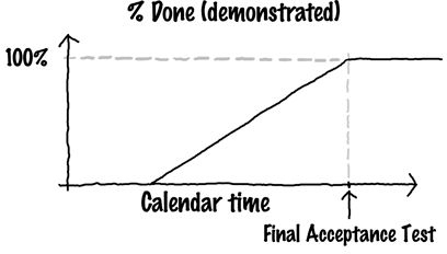
If you now go about system construction in a pure “big bang” approach (build all the pieces, integrate and test them all, deliver them all when ready), then your only metric of doneness is the final acceptance test. As a function of time, your demonstrated doneness would look like this:

You give evidence of being 0-percent done until the very end, when you’re suddenly 100-percent done. The only reason you have for believing otherwise (say, for believing at some point that you’re 50-percent done) is soft evidence.

EVR is intended to give you objective evidence of partial doneness, something that will allow you to draw—and believe in—a picture like this:

There will still be a period early in the project when progress is supported only by faith. However, from well before the project midpoint, you should be obtaining some credible EVR evidence of partial doneness.

EVR depends on your ability to build the system incrementally, say by implementing selected subsets of the system’s pieces, called versions. So Version 1, for example, might be the following:

Here, you’ve connected (as best you can) the net inflows and out-flows to the partial product. Of course, the partial system can’t do all of what the full system does, but it can do something—and that something can be tested. So you test it. You construct a Version 1 acceptance test, and when it passes, you declare that portion of the whole to be done.

Version 2 adds functionality:

It, too, gets its own acceptance test. When it passes the test, you declare that much of the system done.

But in each case, how much is “that much”? Our brief answer is EVR, the “earned value” of the running segment. It’s the portion of the whole budget that you have now “earned” credit for by demonstrating completion. (See Chapter 16 for details on computing EVR.)

If you can break up implementation into perhaps ten versions, you should be able to calculate in advance the EVR for each one and produce a table like this:

Now, from the time V1 passes its version acceptance test (VAT1), you will be able to plot a curve showing the expected date of each subsequent VAT. As the tests are passed, you can track expected versus actual EVR in this form:

Manifestation of any of the core risks (or any major risk, for that matter) will cause marked lagging of the actual versions completed, behind the expected.

The example we’ve shown here is clearly concocted. But in choosing the numbers and the shape of the actual-versus-expected graph, we’ve tried to give you a sense of the approximate degree of control the scheme will provide.