4. Formatting Worksheet Data

In this chapter, you explore the various types of formatting you can apply to both your cells and your data. The topics in this chapter include
→ Changing the font, font size, and font style
→ Changing column width and row height
→ Changing the background and text color
→ Modifying data alignment and cell orientation
→ Clearing and copying formatting
→ Hiding rows, columns, and worksheets
→ Creating and applying a formatting style
→ Using conditional formatting
The primary purpose of Excel’s formatting tools is to make your worksheet more readable. For example, you can change the display of the numbers so that they don’t contain decimal places. This enables your audience to see the needed data without being inundated with superfluous numbers.
Excel’s formatting options can be partitioned into two buckets: cell formatting and data formatting.
Cell formatting changes the look and feel of the cells. For instance, you can change the cell background colors, add borders, change alignment, add underline or bold effects to cell contents, and wrap text.
Data formatting changes the data to the most readable and appropriate way. For example, you can format a number to show as currency complete with the dollar symbol. Or you can format a date so that is shows as Jan-14 instead of 01/01/2014.
Changing the Font and Font Size
One way to format data in your worksheet is to change the font used to display it. This gives data a different look and feel, which can help differentiate the type of data a cell contains. You can also change the font’s size for added emphasis.
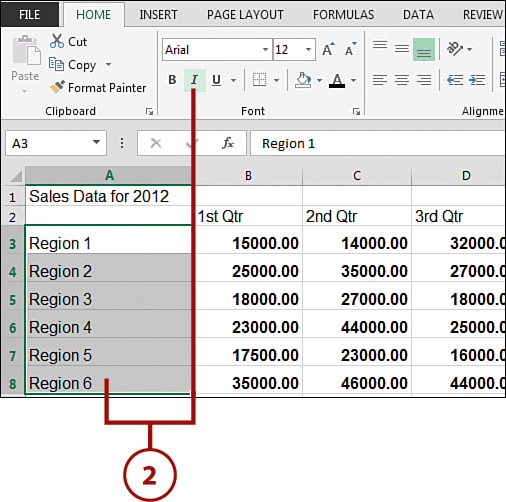
1. Select the cells whose font and font size you want to change, or click the All Cells button (to the left of column A and above row 1) to format all the cells in the worksheet.

2. Click the Font field down arrow on the Home tab, and scroll through the available fonts. When you find the one you want to use, click it to select it.
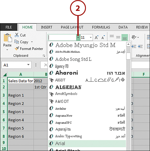
Finding Font Names
If you know the name of the font you want to apply, select the down arrow next to the Font field, and type the first letter of the font name. You are immediately moved to the portion of the list that starts with the typed letter.
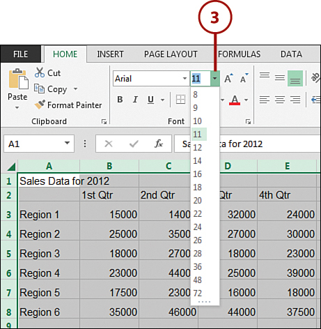
3. Click the Font Size field down arrow and scroll through the available sizes (in points). When you find the size you want to use, click it to select it.
4. Note that the font and font size you selected are applied.
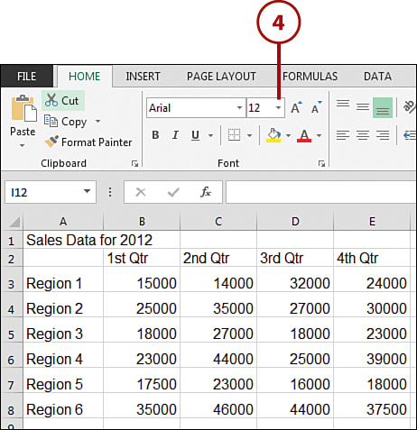
Formatting Options
To format only a portion of a cell’s data, select only that portion and then change the font. You can also select a font (or other options) before you begin typing, and all the data in that cell appears with the selected font or options.
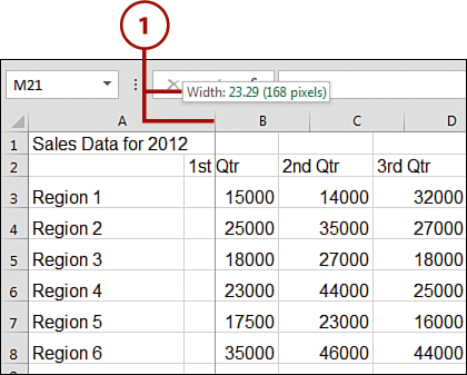
Changing Column Width
There might be times when data is too wide to display within a cell, particularly if you just applied formatting to it. Excel provides several alternatives for fixing this problem. You can select columns and specify a width or force Excel to automatically adjust the width of a cell to exactly fit its contents.
1. Move the mouse pointer over one side of the column header; then click and drag the column edge to the wanted width. (The column size displays in the Name box.)
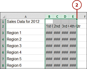
2. To resize multiple columns simultaneously, select the columns that you want to alter.
3. Click and drag one of the selected columns’ header edges to the wanted width and release it.
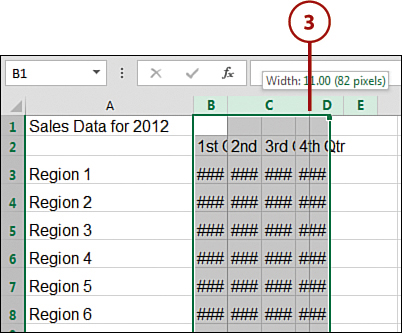
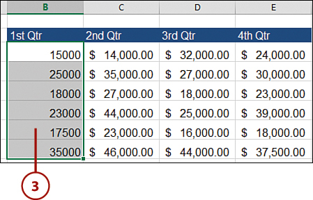
4. All the selected columns are resized to the same width.

Quick AutoFit Column Widths
Here’s a quick and easy way to automatically make all columns fit their individual contents. Select the columns you want to alter, move the cursor over the right side of the column header, and double-click when the cursor changes to a two-headed arrow. Your columns automatically snap tightly around their contents.
Changing the Color of the Cell Background and Cell Text
Generally, cells present a white background for displaying data, but you can apply other colors or shading to the background. You can even combine these colors with various patterns for a more attractive effect. In addition, you can change the color of the data contained within your worksheet’s cells.
1. Select the cells whose background color and/or font color you want to change.

2. To change the color of the text in the selected cells, click the Font Color down arrow on the Home tab, and choose a color from the list (here, white).

3. To change the color of the selected cells’ background, click the Fill Color down arrow, and choose a color from the list (here, blue). Excel applies the colors.

Choosing Colors
Be sure a shading or color pattern doesn’t interfere with the readability of your data. To improve readability, you might need to make the text bold or select a text color that goes well with your cells’ background color.
Think of the Printer
If you print the worksheet to a noncolor printer, the color you select prints gray—and the darker the gray, the less readable the data. Yellows generally print as a pleasing light gray that doesn’t compete with the data.
Formatting the Display of Numeric Data
You can alter the display of different numbers depending on the type of data the cells contain. By formatting numeric data, you can display data in a familiar format to make it easier to read. For example, sales numbers can display in a currency format, and scientific data can display with commas and decimals.
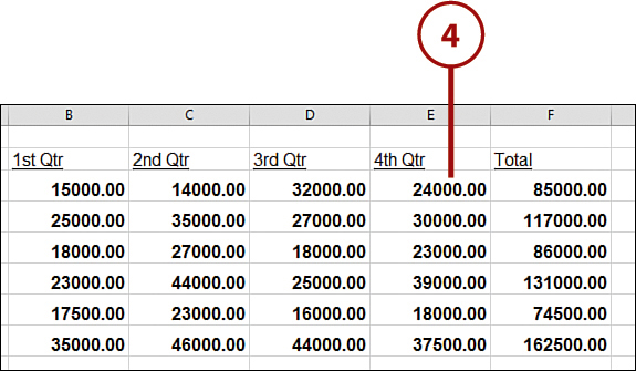
1. After you select the cells you want to format, click the Increase Decimal command on the Home tab twice (once for each decimal place you want displayed).

2. Click the Comma Style command on the Home tab to add a comma to the numeric data.

3. Click the Accounting Number Format command on the Home tab to format numbers in the selected cells with a dollar sign ($), commas, a decimal point, and two decimal places.

Percent Style
If you click the Percent Style command on the Home tab, your numbers convert to a percentage and display with a % symbol.
Handling the #### Error
After you apply a style to cells, if any cells display the error #########, it simply means that the data in the cell exceeds the current cell width. Refer to the task “Changing Column Width” in Chapter 2, “Managing Workbooks and Worksheets,” to fix the problem.
Use a General Format
When you enter numbers into Excel cells, the General format is the default. No specific number format (discussed in the next task) is applied. The General format is used when you record counts of items, increment numbers, or do not require any particular format. If you have applied another format to your cells but want to return to this default General format, follow the steps in this task.
1. After you select the cells you want to format, click the down arrow in the Number Format drop-down box (on the Home tab).
2. Click the General option in the Category list.

3. Excel changes the format.
Use a Number Format
When you apply the Number format in Excel, it uses two decimal places by default. You have the option to alter the number of decimal places, use a comma separator, and even determine the way you want negative numbers to appear (for example, with a minus sign, in red, in parentheses, or some combination of the three).
1. After you select the cells you want to format, click the down arrow in the Number Format drop-down on the Home tab.
2. Click the Number option in the Category list.
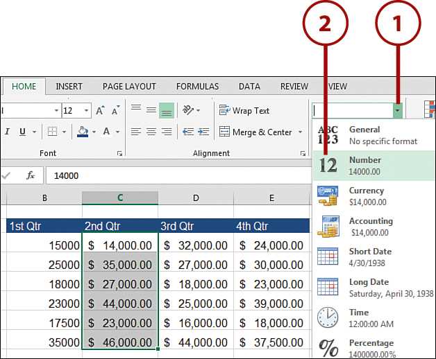
3. Excel changes the format.

Quickly Increase and Decrease Decimal Places
In the Number group on the Home tab are the Increase Decimal and Decrease Decimal commands. These commands enable you to quickly change the number of decimal places used in your values.
Use a Currency Format
When you apply the Currency format in Excel, it uses two decimal places and a dollar sign by default. You have the option to alter the number of decimal places, display a symbol for a different currency, and even determine the way you want negative numbers to appear.
1. After you select the cells you want to format, click the down arrow in the Number Format drop-down box on the Home tab.
2. Click the Currency option in the Category list.
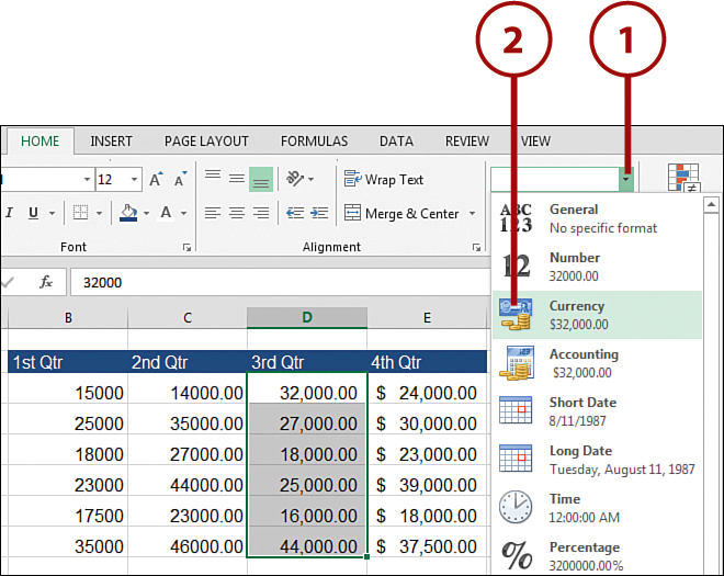
3. Excel changes the format.

Currency Format Options
Use the Decimal Places field in the Number tab of the Format Cells dialog box to change the number of decimal places used. To choose a different currency symbol, select it from the Symbol drop-down list.
Currency-Related Formats
The Accounting format automatically lines up the currency symbols and decimal points for the cells in a column. The Percentage format multiplies the cell value by 100 and displays the result with a percent symbol.
Use a Date Format
When you apply the Date format in Excel, it displays the date and time serial numbers as date values. There are numerous date types you can assign to your dates. For example, you might find it easier to skim through dates as numbers with or without the assigned year visible. Or perhaps you would rather use the actual name of the month (as opposed to a numeral) for reference.
1. After you select the cells you want to format, go to the Home tab, and click the down arrow in the Number Format drop-down box.
2. Click the Short Date option in the Category list.
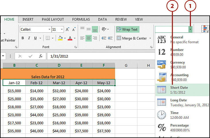
3. Excel changes the format.

You can use the Time format if you want to display just the time (not the date) in your spreadsheet. In addition, you can use the Custom format option (in the Format Cells dialog box) to create your own Date and Time format.
Use a Text Format
When you type numeric data into a cell, the display defaults to a Number format. When you apply the Text format in Excel, it displays numbers as text regardless of whether the data in the cell is numeric or text-based. This can be convenient when you want to enter a number that isn’t meant to be calculated or used in a mathematical operation. For example, you might need to enter a customer number that has leading zeros. Formatting this number as text ensures that the leading zeroes remain visible.
1. After you select the cells you want to format, click the down arrow in the Number Format drop-down box (on the Home tab).
2. Click the Text option in the Category list.

3. Excel changes the format.

Immediate Number Text
Another way to immediately make a number a textual cell entry is to type an apostrophe (‘) before you type the number. This tells Excel that the number is to be treated as text.
Applying Bold, Italic, and Underline
You can format the data contained in one or more cells as bold, italic, or underlined (or some combination of the three) to draw attention to it or make it easier to find. Indicating summary values, questionable data, or any other cells is easy with this type of formatting.
1. Select the cells in which you want to apply bold formatting, and click the Bold command.
2. Select the cells in which you want to apply italic formatting, and click the Italic command.
3. Select the cells in which you want to apply underline formatting, and click the Underline command.

4. The bold, italic, and underlining are applied to the selected cells.
Combination Formatting
You can use several formatting techniques in combination, such as applying bold, italic, and underlining at the same time. Simply select the text you want to format, and click each of the commands on the Home tab.
Using Merge and Center on Cells
Using Excel’s Merge and Center feature, you can group similar data under one heading. Columns of data usually have column headers, but they can also have group header information representing multiple columns.
1. Select the cells you want to merge, including the cells that don’t contain any data.
2. Click the Merge and Center command on the Home tab.
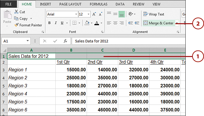
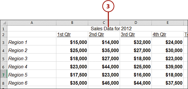
3. The cells in the group header are merged, and the data is centered. Repeat the steps in this task as needed to group additional columns in your worksheet.
Unmerging Cells
To unmerge or separate cells that have been merged, place your cursor in the merged cell; then go to the Home tab and click the Merge and Center command.
Changing Horizontal Data Alignment
Excel provides several ways to format data, and one way is to align it. The most common alignment changes you make will probably be to center data in a cell, align data with a cell’s right edge (right-aligned), or align data with a cell’s left edge (left-aligned). The default alignment for numbers is right-aligned; the default alignment for text is left-aligned.
1. Select the cells in which you want to align the data to the left, and click the Align Left command on the Home tab.
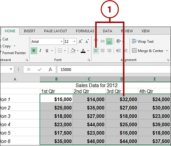
2. Select the cells in which you want to align the data to the right, and click the Align Right command.

3. Select the cells in which you want to center the data, and click the Center command.
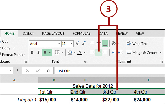
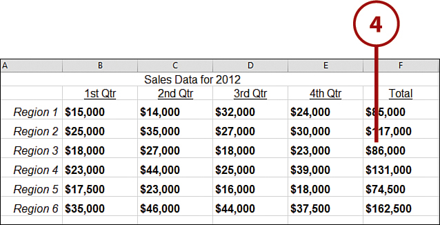
4. The alignments are applied to the selected cells.
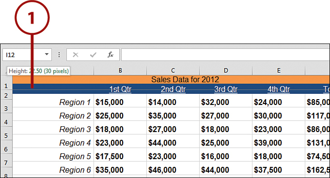
Changing Row Height
Depending on the formatting changes you make to a cell, data might not display properly. Increasing the font size or forcing data to wrap within a cell might prevent data from being entirely displayed or cause it to run over into other cells. You can frequently avoid these problems by resizing rows.
1. Move the mouse pointer over the bottom edge of the row header. Click and drag the row to the wanted height; the row size displays in the bubble.
2. To resize multiple rows simultaneously, select the rows you want to alter.

3. Click and drag one of the selected row’s bottom edges to the wanted height and then release it. All the selected rows are resized to the same height.
Quick AutoFit Rows
Here’s a quick and easy way to automatically make all rows fit their individual contents: Select the rows you want to alter; then move the cursor over the top border of any of the row numbers, and double-click when the cursor changes to a two-headed arrow. Your rows automatically snap tightly around their contents.
Changing Vertical Data Alignment
In addition to aligning the data in your cells horizontally, you can align your cell data in a vertical format. Perhaps you want the data in your cells to align to the top of the cell, the bottom of the cell, or the center of the cell, or you want the data to justify within the cell. Cell data defaults to the bottom of the cell, but you can change this according to the look you want.
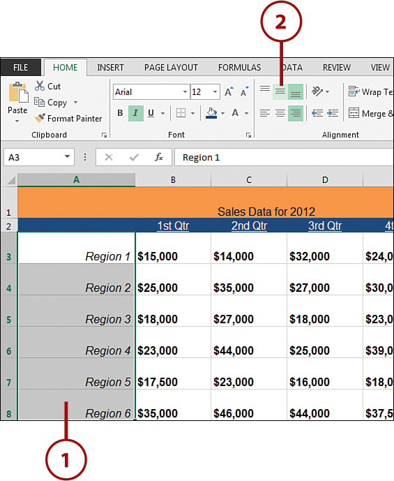
1. Select the cells in which you want to align the data.
2. Go to the Home tab, and click the Middle Align command.
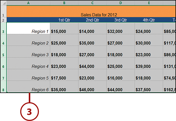
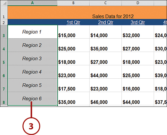
3. The data is vertically aligned within the cell.
Changing Cell Orientation
Excel enables you to alter the orientation of cells—that is, the angle at which a cell displays information. The main reason for doing this is to help draw attention to important or special text. This feature can be convenient when you have a lot of columns in a worksheet and you don’t want your column headers to take up much horizontal space, or if you simply want the information to stand out.
1. After you select the cell or cells whose orientation you want to change, click the Orientation command in the Alignment group on the Home tab.
2. Choose Angle Counterclockwise (shown here) or Angle Clockwise.
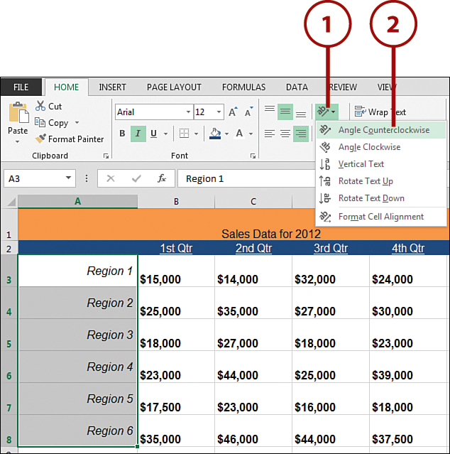
3. The data reorients within the cell. (You might need to increase or decrease the height and width of the cells.)

More Control over Rotating Data
Although the Orientation command gives you an easy way to alter the orientation of your cells, you might need a bit more control over the angle of the orientation. You can define your own orientation angles by right-clicking any cells and selecting Format Cells. In the Format Cells dialog box that appears, go to the Alignment tab. There you see a section called Orientation containing a half-circle. You can rotate the text in the target cell by clicking the red dot there and dragging it to the wanted angle.
Wrapping Data in a Cell
Another way to format data is to allow text to wrap in a cell. For example, suppose a heading (row or column, for example) is longer than the width of the cell holding the data. If you want to make your worksheet organized and readable, it is a good idea to wrap the text in the heading so that it is completely visible in a cell.
1. After you select the cell or cells whose text you want to wrap, click the Wrap Text command in the Alignment group on the Home tab.
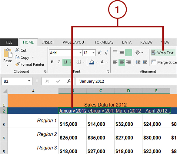
2. The data in the selected cells is automatically wrapped and the cell height adjusts.

Aligning Wrapped Text
You might need to alter the column width to have the data wrap at the location you want. You also can align data that has been wrapped, which gives your text a cleaner look. Refer to the tasks “Changing Horizontal Data Alignment” and “Changing Vertical Data Alignment” earlier in this chapter to learn how to align data in cells.
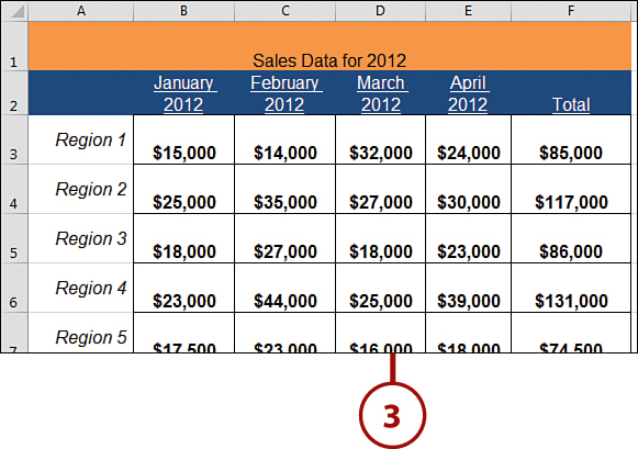
Changing Borders
Each side of a cell is considered a border. Borders provide a visual cue as to where a cell begins and ends. You can customize borders to indicate other beginnings and endings, such as grouping similar data or separating headings from data. For example, a double line is often used to separate a summary value from the data being totaled. Changing the bottom of the border for the last number before the total accomplishes this effect.
1. Select the cells to which you want to add some type of border.
2. On the Home tab click the down arrow next to the Borders command, and then choose an option from the list that appears—for example, All Borders.
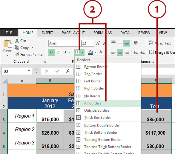
3. The border is applied.
Removing Borders
To remove a border, select the bordered cells, click the down arrow next to the Borders command, and choose the No Border option from the list that appears.
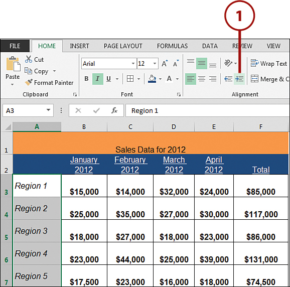
Indenting Entries in a Cell
Another alignment option you might want to use is to indent entries within a cell. Doing so can show the organization of entries—for example, subcategories of a budget category.
1. After you select the cell or range whose data you want to indent, click the Increase Indent command the number of times you want the entries indented.
2. To decrease the indent, select the cell or range whose indent you want to decrease.
3. Click the Decrease Indent command to decrease the number of indents.

4. The indentation is decreased.

Increasing Column Width
To make the effect of the indentation stand out, you might need to increase the width of the indented column. To do so, refer to the task “Changing Column Width” earlier in this part.
Clearing Formatting
Excel enables you to quickly clear all the formatting you have added to cell data, returning numbers and text to their original format.
1. Select the cells whose formatting you want to clear.
2. On the Home tab, click the down arrow next to the Clear command, and then choose Clear Formats.
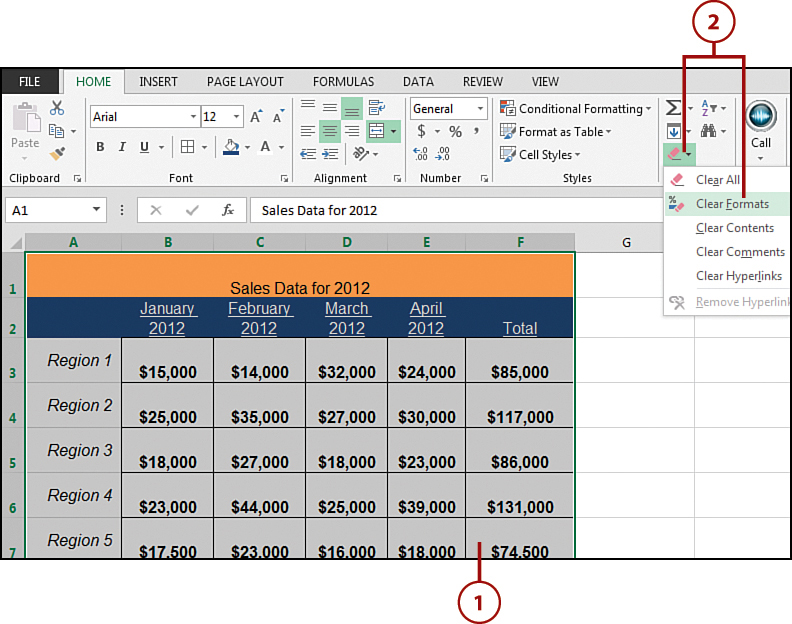
3. The cell data remains, but all the formatting is gone.
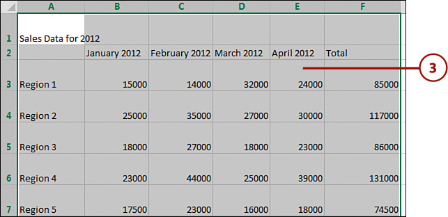
If you choose Clear Contents, the formatting remains intact, but the text and data (contents) are deleted (just as if you simply pressed the Delete key on the keyboard). If you choose Clear All, all the formatting and contents (and comments) are removed from the cell.
Hiding and Unhiding Rows
Hiding rows is a good way to hide calculations that aren’t critical for your audience to see. You also can hide other rows that you want to include in the worksheet but don’t want to display. It’s tricky to unhide a row because you need a way to select the hidden row. This task shows you how.
1. Click any cell in the row, or click the whole row that you want to hide.
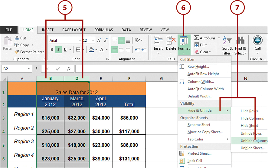
2. Click the drop-down arrow next to the Format command on the Home tab.
3. Select Hide & Unhide and then click Hide Rows.

4. You can tell when a row is hidden by the nonsequential jump in the row numbers. For instance, if row 5 is hidden, you see rows 3, 4, 6, 7, and so on.
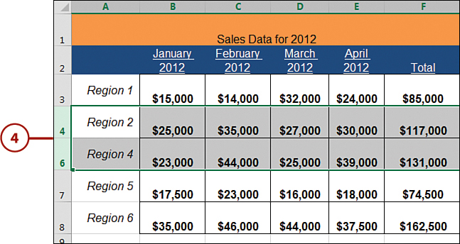
5. To unhide the row, select the rows above and below the hidden row.
6. Click the drop-down arrow next to the Format command on the Home tab.
7. Select Hide & Unhide and then click Unhide Rows.

Printing Hidden Elements
Hidden elements, whether they’re rows, columns, or worksheets, don’t print when you print the worksheet.
Every row has a top border and bottom border (the lines that separate the row numbers). You can click and drag any row’s bottom border to either make the row taller or shorter depending on which direction you drag it (up or down). If you drag the bottom border of a row so that it is touching its top border, you can see that the row is effectively hidden. That is to say, you can drag the bottom border of a row so that it is practically zero height.
Hiding and Unhiding Columns
Hiding columns is a good way to hide calculations that aren’t critical for your audience to see. You also can hide columns that you want to include in the worksheet but don’t want to display. It’s tricky to unhide a column because you need a way of selecting the hidden column. This task shows you how.
1. Click any cell in the column, or click the whole column that you want to hide.
2. Click the drop-down arrow next to the Format command on the Home tab.
3. Select Hide & Unhide and then click Hide Columns.

4. You can tell when a column is hidden by the nonsequential jump in the column letters. For example, if column C is hidden, you see columns A, B, D, and so on.
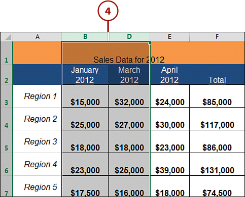
5. To unhide the column, select the columns to the left and right of the hidden column.
6. Click the drop-down arrow next to the Format command on the Home tab.
7. Select Hide & Unhide and then click Unhide Columns.
Every column has a left border and right border (the lines that separate the column letters). You can click and drag any column’s right border to either make the column wider or more narrow depending on which direction you drag it (left or right). If you drag the right border of a column so that it touches its left border, you can see that the column is effectively hidden. That is to say, you can drag the right border of a column so that it is practically zero width.
Hiding and Unhiding a Worksheet
Often, you might have worksheets that are meant for your eyes only. An example of this would be a worksheet where you document changes in the workbook over the course of development. This kind of worksheet would be administrative in nature and not meant for your audience. In this scenario, hiding the worksheet would be ideal.
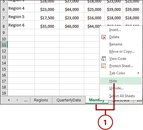
1. After you select the tab of any sheet you want to hide, right-click the tab and choose Hide. Excel hides the sheet.
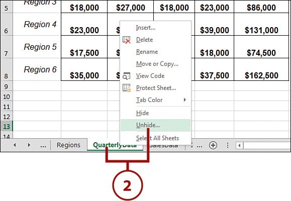
2. To unhide the sheet, right-click any tab and choose Unhide.
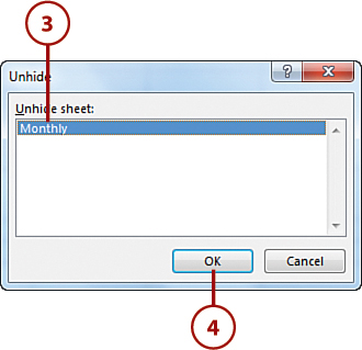
3. The Unhide dialog box opens, listing sheets that are hidden in your workbook. Click the worksheet name you want to unhide.
4. Click the Ok button.
A Hidden Sheet Is Not a Protected Sheet
Be aware that savvy users will know how to look for and unhide your hidden sheets. Do not count on hidden sheets to reliably protect sensitive information. For data protection, consider password protecting your workbook as shown in Chapter 2.
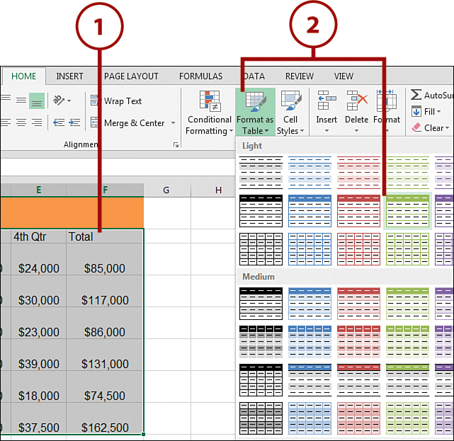
Using Format as Table
Using all the formatting capabilities discussed to this point, you could format your worksheets in an effective and professional manner—but it might take a while to get good at it. In the meantime, you can use Excel’s Format as Table feature, which can format selected cells using predefined formats. This feature is a quick way to format large amounts of data and provides ideas on how to manually format data.
1. Select the cells to which you want to apply Format as Table.
2. Click on the down-arrow next to the Format as Table command (found on the Home tab); then scroll through the available formats, and click the one you want to apply to your data.
3. Click OK on the next pop-up to confirm that the selected range is correct.

4. The AutoFormat is applied.

Modifying Format As Table
If you go to the Design tab and then run your cursor over the different styles in the Table Styles group, the selected ranges change accordingly so that you can see a preview of what that style does to the data.
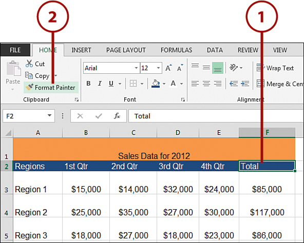
Copying Formatting
If you have formatted a specific cell as you want, you might decide to apply those same formatting options to other cells. Instead of repeating each step in the format process over and over again, you can simply use the Format Painter command.
1. Click the cell with the formatting that you want to copy and apply to other cells.
2. Click the Format Painter command on the Home tab; the mouse pointer changes to a Format Painter pointer (paint-brush symbol).
3. Click and drag the mouse pointer to select the cells to which you want to apply the copied formatting.
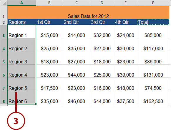
4. Release the mouse button. The formatting is applied to the data in the selected cells.

Make Format Painter Persist
Double-click the Format Painter command (instead of single-clicking) and the Format Painter remains active, enabling you to format multiple areas without the need to constantly reactivate it. To turn Format Painter off, simply click it again, or press the Esc button on the keyboard.
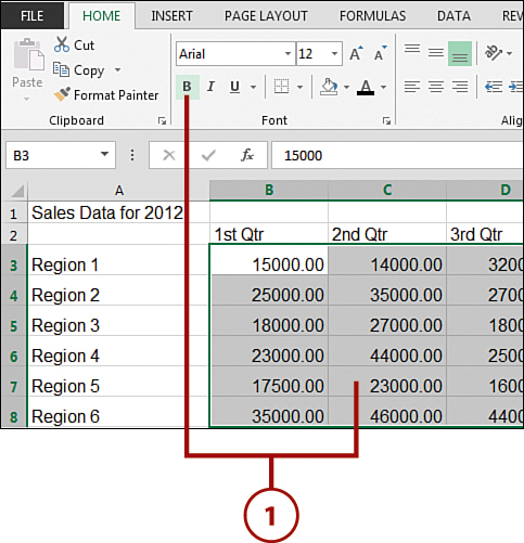
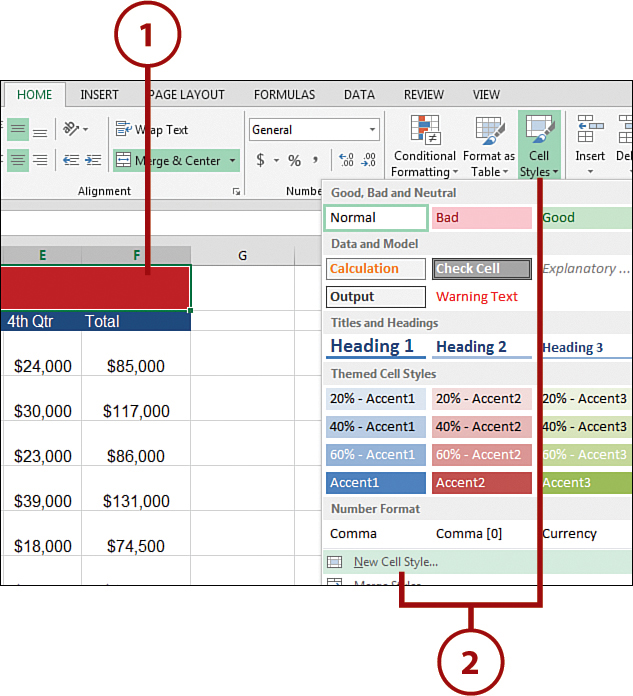
Creating and Applying a Formatting Style
Instead of assigning your data an existing Excel style (for example, Normal, Currency, Percent, and so forth), you can create your own style and apply it to cells. Begin by applying the specific formatting (for example, font, font style, font size, font color, and cell color) that you want the style to have, and then give the style a specific name.
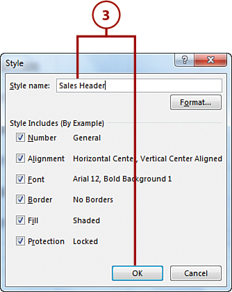
1. Apply any specific cell formatting that you want the style to use in your worksheet (here, Arial, Bold, 12 pt, White text, and Red fill color).
2. With the cell that contains the wanted formatting selected, click the down arrow next to the Cell Styles command on the Home tab. Here, you can see Excel’s Cell Styles gallery with all the default styles. Go to the bottom and choose New Cell Style.
3. Type a descriptive name for the new style in the Style name field (for example, Sales Header) and click OK. Your new style displays with the default styles in the Cell Styles gallery.
Saving the Style
The next time you exit Excel, you are notified that you made a change to your global template and are asked if you want to save the changes. If you want to keep the style you just created, click the Yes button; otherwise, click the No button.
4. Select the cells to which you want to apply your newly created style.
5. Click the down arrow next to the Cell Styles command on the Home tab, and then choose your custom style in the Custom style group at the top.
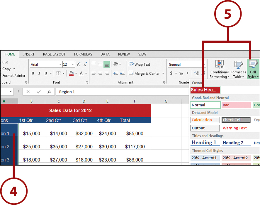
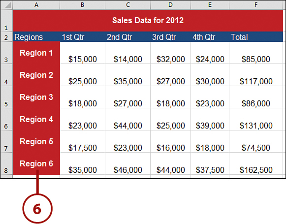
6. The style is applied to the cells you selected.
Default Styles
There are also default styles for Data and Model, Titles and Headings, Themed Cell Styles, and Number Format. You can run your cursor over each option to see how it changes your data prior to selecting it.
Using Conditional Formatting
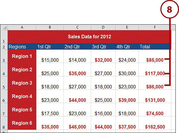
There might be times when you want the formatting of a cell to depend on the value it contains. For this, use conditional formatting, which enables you to specify conditions that, when met, cause the cell to be formatted in the manner defined for that condition. If none of the conditions are met, the cell keeps its original formatting. For example, you can set a conditional format such that if sales for a particular month are greater than $30,000, the data in the cell is bold and red.
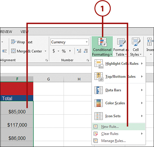
1. Select the cells to which you want to apply conditional formatting; then click the down arrow next to the Conditional Formatting command on the Home tab, and choose New Rule.
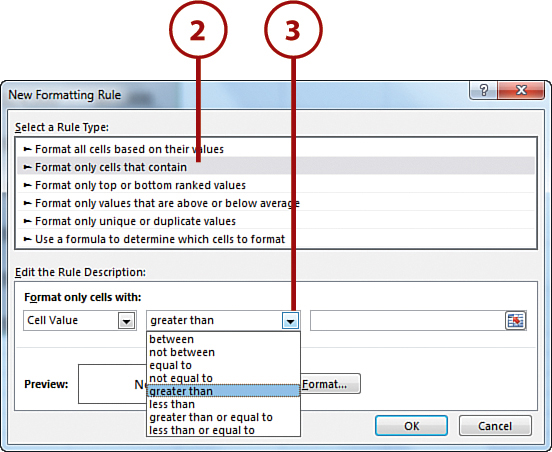
2. In the New Formatting Rule dialog box, choose the Format Only Cells That Contain option.
3. Leave the first drop-down list as Cell Value. Open the second drop-down list to select the type of condition (for example, Greater Than).
Painting a Format onto Other Cells
You can copy the conditional formatting from one cell to another. To do so, click the cell whose formatting you want to copy; then click the Format Painter command. Finally, drag over the cells to which you want to copy the formatting.
4. Type the value of the condition (the number that the cells must be “greater than”).
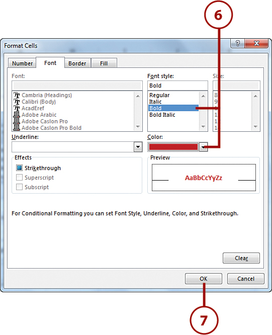
5. Click the Format command to set the format to use when the condition is met.

6. Click the options you want to set in the Format Cells dialog box (for example, Red in the Color field and Bold in the Font style list), and click OK.
7. Click OK in the Format Cells dialog box.
8. Excel applies the formatting to any cells that meet the condition you specified.
When to Use Conditional Formatting
Use conditional formatting to draw attention to values that have different meanings, depending on whether they are positive or negative, such as profit and loss values.