5. Working with Formulas and Functions

This chapter walks you through the ins and outs of using Excel formulas and functions. By the end of this chapter, you will be well equipped to start building your own formulas!
→ Entering and editing a formula
→ Assigning names to a cell or range
→ Working with functions
→ Recognizing and fixing errors
→ Checking for formula references (PRECEDENTS)
→ Checking for cell references (DEPENDENTS)
A formula is essentially a series of instructions you give Excel to return a value. These instructions can be mathematical operations, or a call to a built-in Excel function. Excel typically displays the result of a formula in a cell as either numeric or textual data.
Functions are abbreviated formulas that perform specific operations on a group of values. Excel provides more than 250 functions that can help you with tasks ranging from determining loan payments to calculating investment returns. For example, the SUM function automatically adds up the numeric values within a given range.
Using AutoSum Calculations
Excel has several built-in formulas that perform the most commonly used calculations for you. These built-in calculations include Sum, Average, Count, Max, and Min. You start your exploration of Excel formulas and functions with these predefined calculations. The most prominent of these is the AutoSum or sum. You’ll probably use the AutoSum formula a lot—it adds numbers in a range of cells.
1. Click in the cell in which you want the result of the AutoSum operation to appear, which is called the resultant cell.
2. Click the AutoSum command on the Home tab.
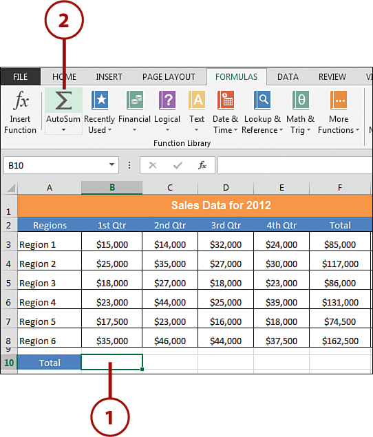
3. Excel selects the most obvious range of numbers and puts a dotted line around the cells. Press Enter to accept the range, or use the mouse to select alternative cells.
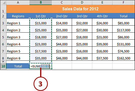
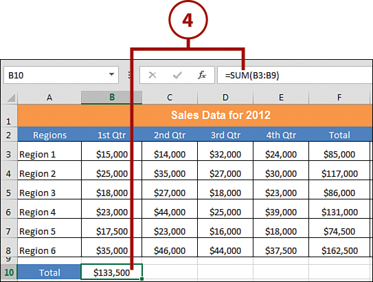
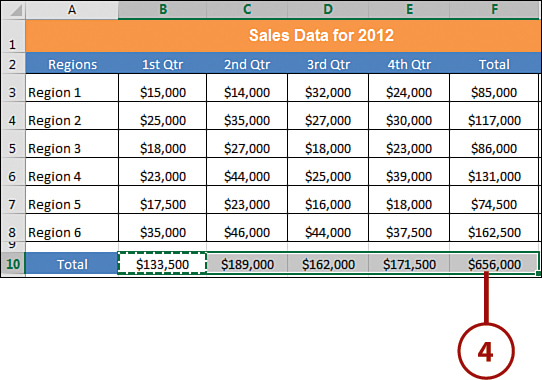
4. Click the resultant cell to make it the active cell. The formula displays on the Formula bar.
AutoSum Shortcut Key
Excel provides an easy way to implement the AutoSum via a shortcut key. Simply go to your keyboard and enter the combination of Alt and the equal sign (=). Excel performs the AutoSum for you. At that point, just press Enter on your keyboard to accept the AutoSum calculation.
Find a Cell Average (AVERAGE)
You can use Excel’s AVERAGE function to determine the average of each quarter per region.
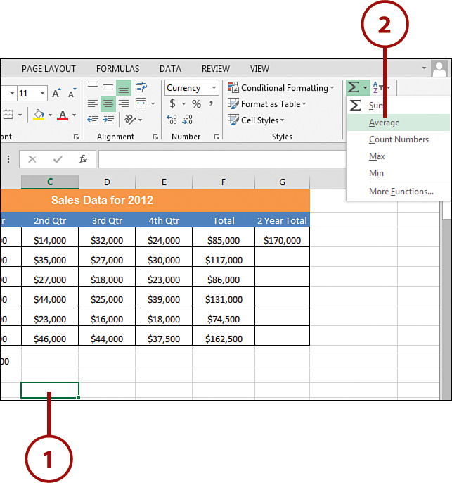
1. Click the cell in which you want the result of the AVERAGE function to appear, which is called the resultant cell.
2. Click the down arrow next to the AutoSum command on the Home tab, and choose Average from the list that appears.
3. Excel selects the most obvious range of numbers and puts a dotted line around the cells. Press Enter to accept the range, or use the mouse to select alternative cells.

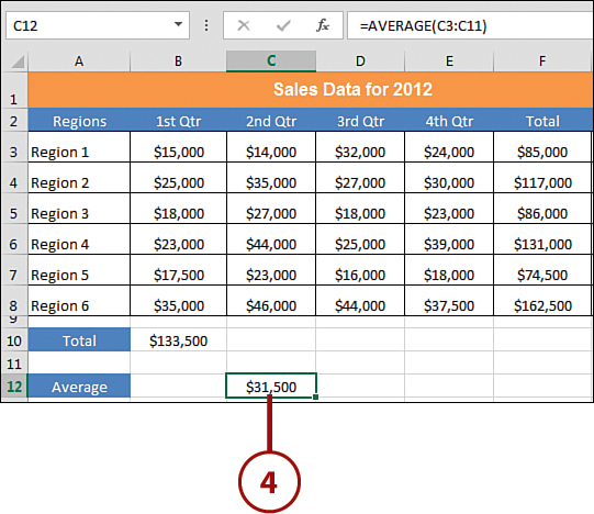
4. Click the resultant cell to make it the active cell. The formula displays on the Formula bar.
Selecting Specific Cells for Your Calculation
If you don’t want to use the range of cells that Excel selects for you, click the first cell you want, hold down the Ctrl key, and click each additional cell you would like to include in the calculation. When you finish selecting the cells you want to calculate, press Enter to see the result. Alternatively, if you let Excel select the cells for you but Excel doesn’t select exactly the right set of cells, you can resize the selection by clicking the first cell to include, holding down the Shift key, and clicking the last cell to include.
Find the Largest Cell Amount (MAX)
As its name suggests, the MAX function returns the largest/maximum number in any given range. You typically use this function if you need to dynamically reference the largest number in other formulas. For example, you can use Excel’s MAX function to determine the quarter in which you had the most sales. Although it’s easy to see this information with your eyes, the Quarter with the most sales changes as each quarter passes. Instead of manually keeping up with which quarter is the king of sales, the MAX function does that for you.
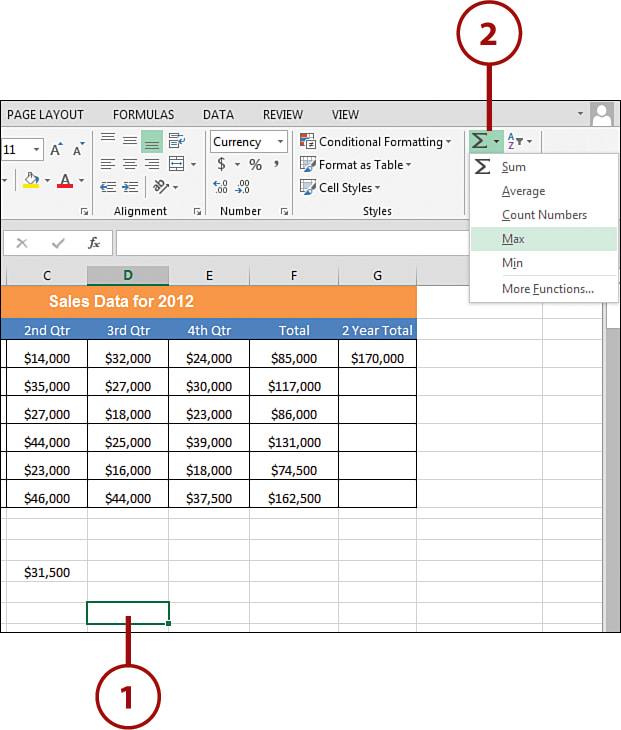
1. Click the cell in which you want the result of the MAX function to appear, which is called the resultant cell.
2. Click the down arrow next to the AutoSum command on the Home tab, and choose Max from the list that appears.
3. Excel selects the most obvious range of numbers and puts a dotted line around the cells. Press Enter to accept the range or use the mouse to select alternative cells.
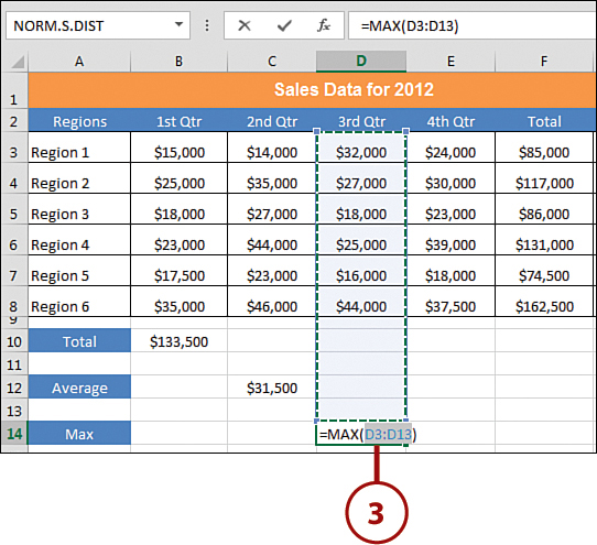
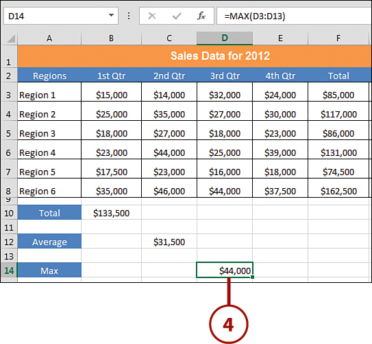
4. Click the resultant cell to make it the active cell. The formula displays on the Formula bar.
Find the Smallest Cell Amount (MIN)
As its name suggests, the MIN function returns the smallest/minimum number in any given range. This is the direct opposite of the MAX function, which returns the largest number in a range. You would typically use Excel’s MIN function to determine the lowest performing Region, or Market, or whatever else you want to measure. This quickly gives you a reference point for the lowest number in your data.
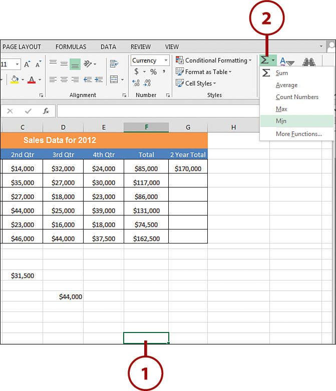
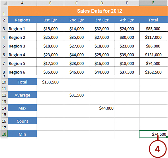
1. Click the cell in which you want the result of the function to appear, which is called the resultant cell.
2. Click the down arrow next to the AutoSum command on the Home tab, and choose Min from the list that appears.
3. Excel selects the most obvious range of numbers and puts a dotted line around the cells. Press Enter to accept the range, or use the mouse to select alternative cells.
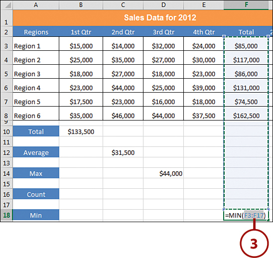
4. Click the resultant cell to make it the active cell. The formula displays on the Formula bar.
Count the Number of Cells (COUNT)
As you might have guessed, the COUNT function literally counts the number of data points in any given range. Suppose you want to know how many values (data points) are in your data table; you can use Excel’s COUNT function to count the number of cells in a selected range.
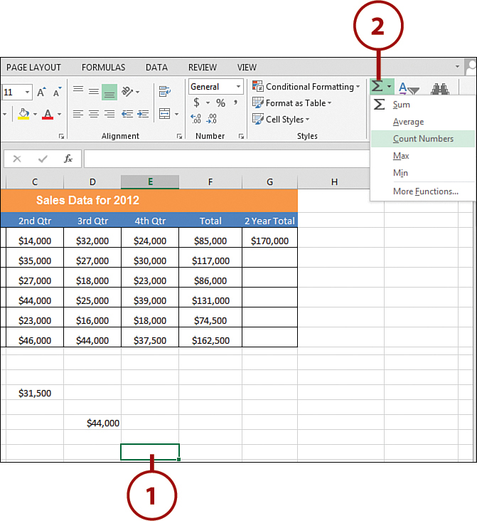
1. Click the cell in which you want the result of the COUNT function to appear, which is called the resultant cell.
2. Click the down arrow next to the AutoSum command on the Home tab, and choose Count Numbers from the list that appears.
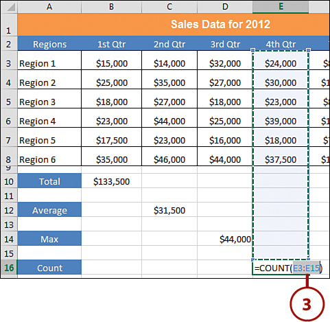
3. Excel selects the most obvious range of numbers and puts a dotted line around the cells. Press Enter to accept the range or use the mouse to select alternative cells.
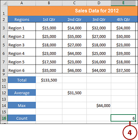
4. Click the resultant cell to make it the active cell. The formula displays on the Formula bar.
Counting Text Values
The COUNT function works only if the range you count is numbers-based. That is, it counts only numeric values (not text). To count the data points in a range that contains text, you can use the COUNTA function. Using the COUNTA function counts both numeric and textual values. To use COUNTA, simply edit your formula by replacing the word COUNT with COUNTA.
Entering a Formula
Another way to use a formula is to type it directly into the cell. You can include any cells in your formula; they do not need to be next to each other. Also, you can combine mathematic operations—for example, C3+C4–D5.
1. Click the cell in which you want the result of the formula to appear, which is called the resultant cell.
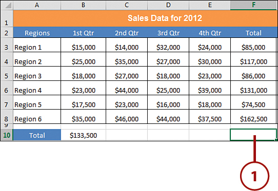
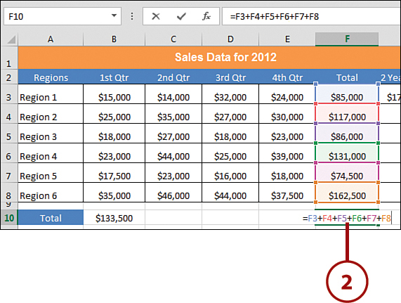
2. Type = (the equal sign) followed by the references of the cells containing the data you want to total (for example, F3+F4+F5+F6+F7+F8). Press Enter.
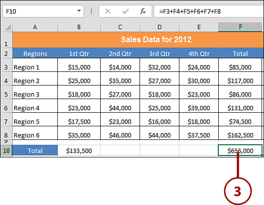
3. Click the resultant cell to make it the active cell; the values in the specified cells are added together.
Editing a Formula or Function
After you enter a formula or function, you can change the values in the referenced cells, and Excel automatically recalculates the result based on the changes. You can include any cells in a formula or function; they do not need to be next to each other.
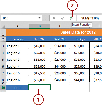
1. Click the cell you want to edit; the function displays on the Formula bar.
2. Click the Insert Function command on the Formula bar to open the Function Arguments dialog box. (If using a formula, the Insert Function dialog box displays.)
3. Type the changes to your function. For example, change the cells being calculated to B3–B8 instead of B3–B9. Click OK.
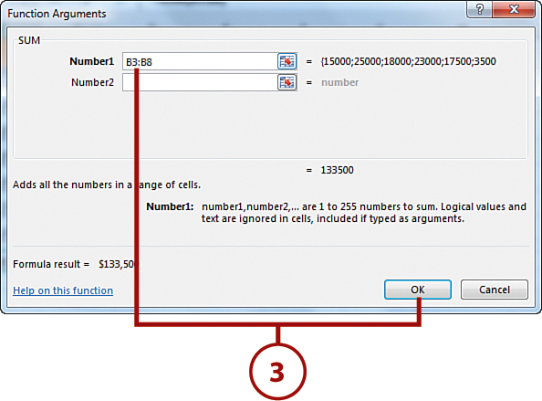
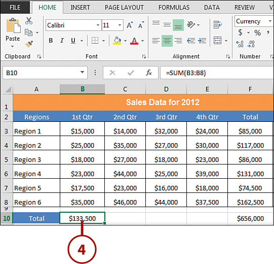
4. The changes are made and the result appears in the cell.
Pressing F2
Instead of using the Function Arguments dialog box to edit your formulas, you can press the F2 key and edit your formula just like you would for regular text or data on the Formula bar.
Copying a Formula
When you build your worksheet, you might want to use the same data and formulas in more than one cell. With Excel’s Copy command, you can create the initial data or formula once and then place copies in the appropriate cells. For example, suppose you want to find the average sales per quarter in other sales regions. To do so, create the formula for the first region and then copy it to cells for the other regions. Excel automatically figures out how to change the cell ranges to which the formula should apply.
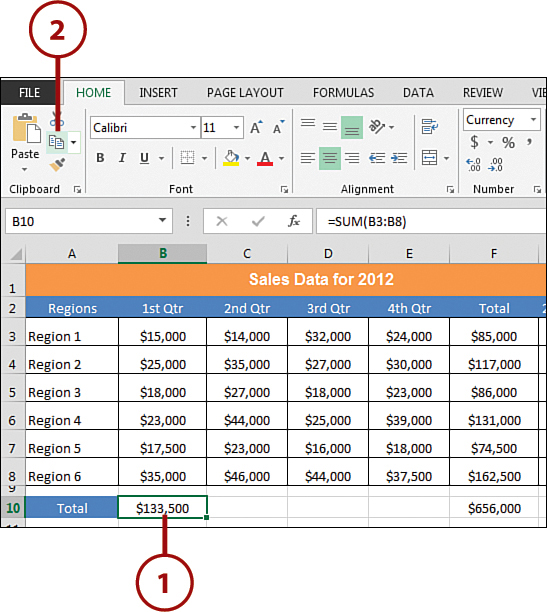
1. Click the cell that contains the function you want to copy.
2. Click the Copy command on the Home tab; a line surrounds the cell you are copying.
3. Click the cell or cells into which you want to paste the formula.
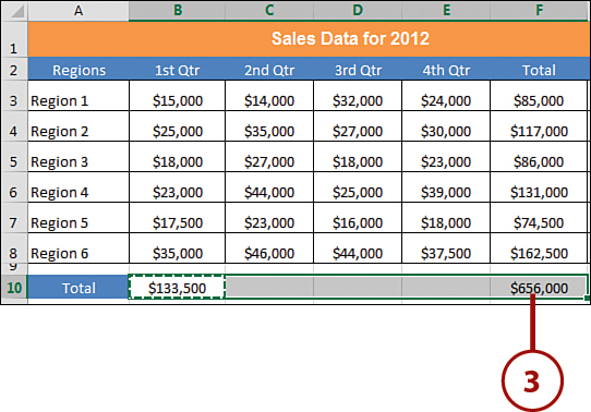
4. Press Enter (or Ctrl+V) to paste the formula into each of the selected cells.
Increasing Cell Width
If you paste a copied formula, you might need to alter the size of your columns to accommodate the new size of the data in the cell. To automatically make an entire column (or multiple columns) fit the width of the widest cell in that column (or columns), move the cursor over the right side of the column header, and double-click when the cursor changes to a two-headed arrow.
Assigning Names to a Cell or Range
You can create range names that make it easier to create formulas and move to that range. For example, a formula that refers to a range named 1stQtr is easier to understand than one named B4:B9. Not only is it easier to remember a name than the cell addresses, but Excel also displays the range name in the Name box—next to the Formula bar. You can name a single cell or a selected range in the worksheet.
1. Select the cell or range you want to name.
2. Click in the Name box; type the wanted range name and press Enter.
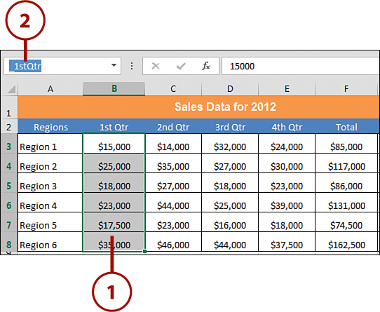
3. Highlight the range and note that the name appears in the Name box.

Referencing Names in a Function
One of the reasons you create a name for a cell or group of cells is so that you can easily refer to that cell or range in a function. That way, rather than typing or selecting a range or cell, you can type the name or select it from the Paste Name dialog box.
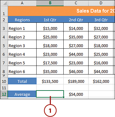
1. Click in the cell in which you want the result of the formula to appear, which is called the resultant cell.
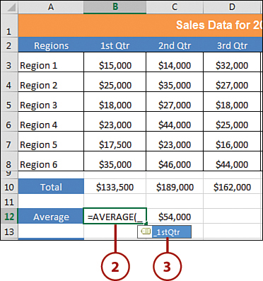
2. Type the function in the cell using a named cell or range—for example, =AVERAGE(_1stQtr). As you type the name, you should see a list of named ranges pop up below the cell.
3. Click a named range to select it.
4. Press Enter and Excel displays the result of the formula.

Quickly Retrieve a Range Name
If you forget the name of a range while you are typing a formula, go to the Formula tab, and click the Use in Formula drop-down. You see a list of the available range names. Simply choose the one you want to use. The range name is automatically placed in the formula.
Deleting a Range Name
To delete a range name, go to the Formulas tab and click the Name Manager. Click the range name you want to get rid of and then click the Delete command. Click OK to confirm the deletion.
Using Functions Across Worksheets
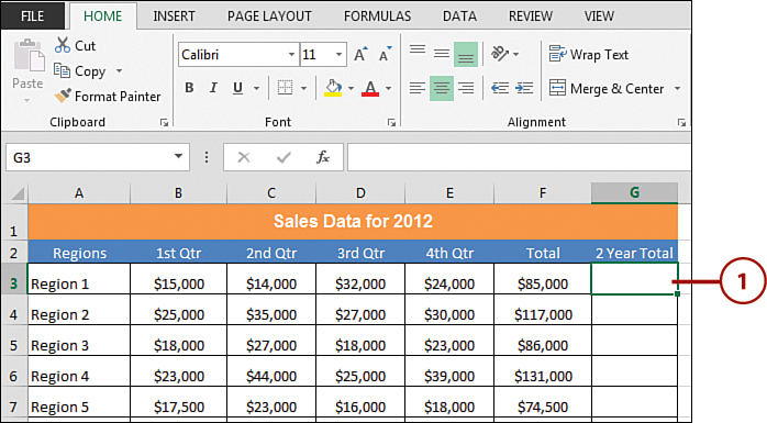
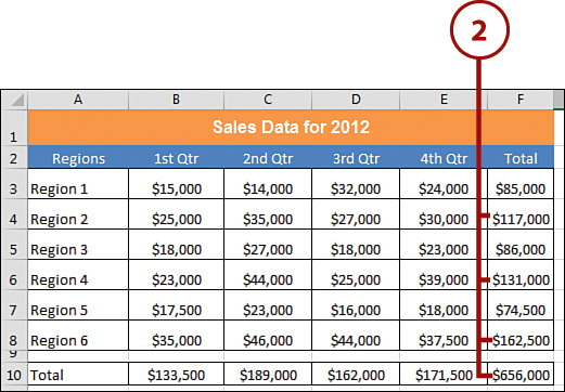
You can use cell references from other worksheets in your calculations. For example, suppose you have two worksheets that contain the calculations for the total sales by region for a particular year. In a third worksheet, you want to calculate the total sales by region for the last 2 years. You can reference the cells in the first two worksheets that contain the totals and perform calculations on them in the third worksheet.
1. Click in the cell in which you want the result of the formula to appear, which is called the resultant cell.
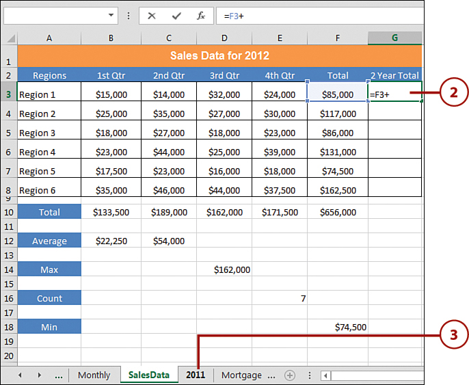
2. This example adds the total for the current year (2012) to last year’s data in another worksheet (2011), so you start the formula by referencing the 2012 total; then you enter a + (plus sign).
3. Click the tab of the worksheet that contains the cell you want to reference in the calculation.
Using Worksheet Name References
Instead of switching back and forth between worksheets, you can manually type the reference to the worksheet name directly in your formulas. Simply use the location of the cell in a particular worksheet (column letter and row number) in addition to the sheet name—for example, Sheet1!A1. If your sheet name contains spaces, you need to enclose your sheet name with single quotes—for example, ‘My Second Sheet’!A1.
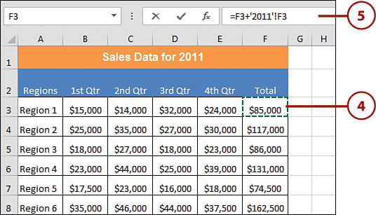
4. Click the cell that you want to use in your calculation; it appears next to the worksheet name on the Formula bar.
5. Press Enter. Excel performs the calculation and returns you to the original worksheet.
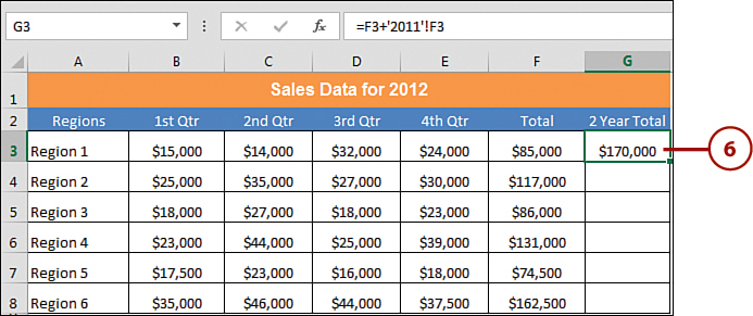
6. Click the resultant cell to make it the active cell. The function displays on the Formula bar.
Be Aware of Worksheet Name References
Each cell you reference from another worksheet must be prefaced with its worksheet name. For example, if you have the formula =SUM(Sheet1!A1+B1) in cell C3 of Sheet2, it references cell A1 from Sheet1 and B1 from Sheet2. If you need to reference both A1 and B1 from Sheet 1, you must include the worksheet name with both cell references, like so: =SUM(Sheet1!A1+Sheet1!B1).
Using Auto-Calculate
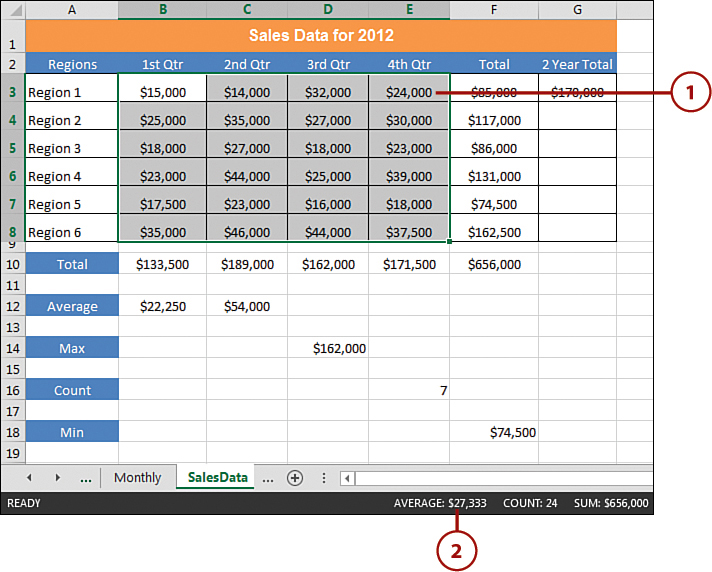
Suppose you want to see a function performed on some of your data—in this example, to determine the lowest quarterly sales goal of any region in 2012—but you don’t want to add the function directly into the worksheet. Excel’s Auto-Calculate feature can help.
1. Select the cells that you want to Auto-Calculate.
2. The Status Bar now shows you the Average, Count, and Sum.
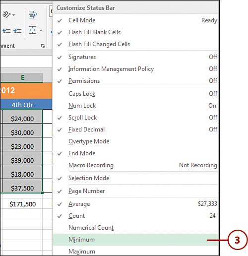
3. Right-click the Status Bar and click each option you want to enable or disable.
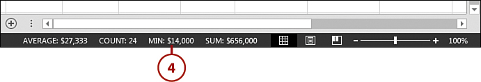
4. Observe your new Auto Calculation(s).
Turning Off Auto-Calculate
You can turn off the Auto-Calculate feature by right-clicking the Status Bar and unselecting each option that is selected.
Finding and Using Excel Functions
In the old days, you needed to know the name of the Excel function you wanted to use. Now, however, Excel makes it easy to find the function you need—all you need to know is what you want the function to do. In the next few tasks, you walk through the creation of several functions using the Insert Function command.
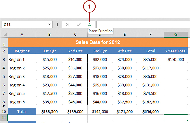
1. Click the Insert Function (fx) command next to the Formula bar.
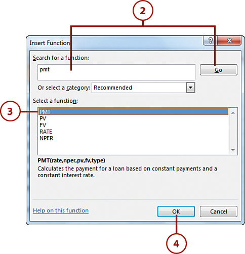
2. Type a description of the function you are looking for in the Search for a Function text box, and press Enter. (Or click the Go button.)
3. Scroll through the list in the Select a Function box and select a function to read a description of it.
4. Click OK after you find the function you want.
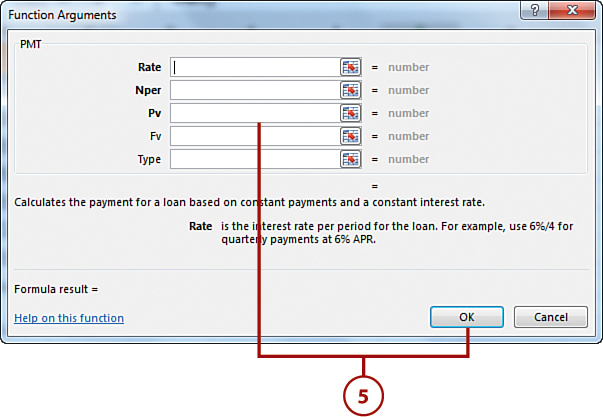
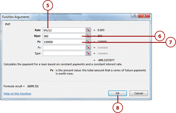
5. Excel walks you through the process of entering the function’s arguments in the Function Arguments dialog box. Click OK when you finish entering its arguments.
Function Arguments Help
If you need help entering your function arguments, click the Help on This Function link in the bottom-left corner of the Function Arguments dialog box.
Calculate a Loan Payment (PMT)
Using Excel, you can determine a monthly loan payment based on a constant interest rate, a specific number of pay periods, and the current loan amount.
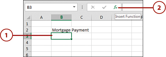
1. Click in the cell in which you want the result of the function to appear, which is called the resultant cell.
2. Click the Insert Function (fx) command next to the Formula bar.
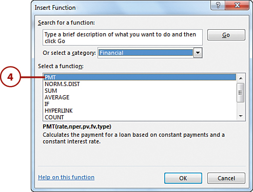
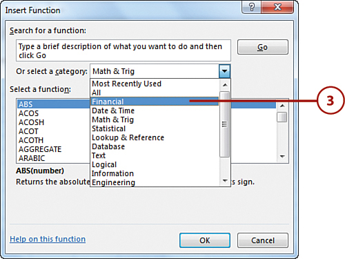
3. The Insert Function dialog box opens. Click the down arrow next to the Or Select a Category field, and choose Financial from the list that appears.

4. A list of financial-related functions appears in the Select a Function list. Scroll through the list to locate the PMT function and double-click it.
Function Arguments Help
If you need help while you are entering your function arguments, click the Help on This Function link in the bottom-left corner of the Function Arguments dialog box.
Your resulting payment is a negative number because payments are considered a debit.
5. In the Rate field, type the interest rate per period. For example, type 6%/12 for monthly payments on a 6 percent annual percentage rate (APR).
6. In the Nper field, type the total number of loan payments. For example, type 360 if you’ll be making 12 payments per year on a 30-year loan.
7. In the Pv field, type the present value of the loan—for example, 150000.
8. Click OK.
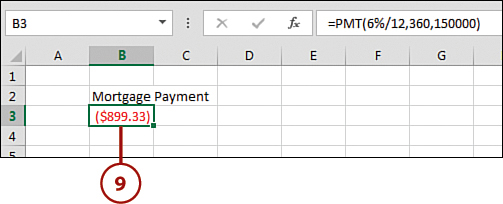
9. Excel calculates the payment and inserts it in the resultant cell.
If you don’t enter a number in the Type argument, it defaults to 0, which means that the last payment pays off the mortgage loan. (This is because mortgages are paid in arrears—at the end of the payment period). If you are calculating a car payment, you might put a 1 in the Type argument because you make your payments at the beginning of the payment period. A 1 versus a 0 makes a slight difference in the calculation because of the interest accrued.
Perform a Logical Test Function (IF)
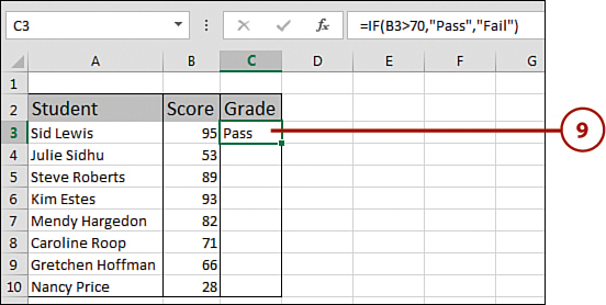
Using Excel, you can perform a logical test function—for example, to indicate whether scores equal a passing or failing grade based on an established set of criteria.
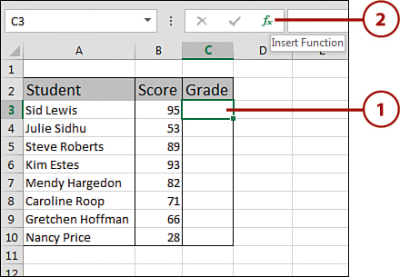
1. Click in the cell in which you want the result of the function to appear, which is called the resultant cell.
2. Click the Insert Function (fx) command next to the Formula bar.
3. The Insert Function dialog box opens. Click the down arrow next to the Or Select a Category field, and choose Logical from the list that appears.
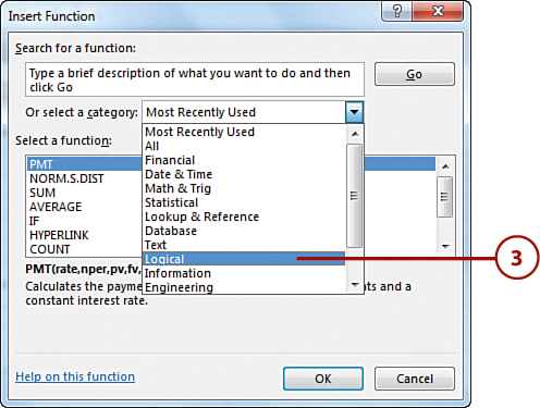
4. A list of logical functions appears in the Select a Function list. Scroll through the list to locate the IF function and double-click it.

Embedded IFs
You can set up embedded IF statements to use in your logical test. For example, suppose scores between 90–100 are an A, 80–89 are a B, 70–79 are a C, 60–69 are a D, and scores 59 and lower are an F. Your formula might look like this: =IF(B3>89, “A”, IF(B3>79, “B”, IF(B3>69, “C”, IF(B3>59, “D”, “F”).
5. In the Logical_test field, type the condition to determine whether a grade is above 70. The logical test is whether the cell is greater than 70; for example, B3>70.
6. In the Value_if_true field, type the value you want to use if the grade is above 70 (that is, a passing grade)—for example, “Pass”.
7. In the Value_if_false field, type the value you want to use if the grade is below 70 (that is, a failing grade)—for example, “Fail”.
8. Click OK.

9. Excel performs the logical test and inserts the result in the resultant cell.
Quick Help with Functions
You can press the F1 key on your keyboard any time you’re typing up an Excel function to automatically be brought to that function’s help screen.
Conditionally Sum a Range (SUMIF)
Using Excel, you can add the data in a range, given certain criteria. This might be useful if, for instance, you need to total the current monthly sales for all sales reps who match a specific criterion—for example, who are all in the same sales region.
1. Click in the cell in which you want the result of the function to appear, which is called the resultant cell.
2. Click the Insert Function (fx) command next to the Formula bar.

3. The Insert Function dialog box opens. Click the down arrow next to the Or Select a Category field and choose Math & Trig from the list that appears.
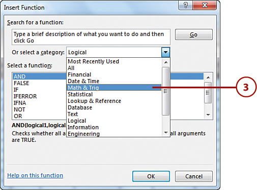
4. A list of math and trig functions appears in the Select a Function list. Scroll through the list to locate the SUMIF function, and double-click it.

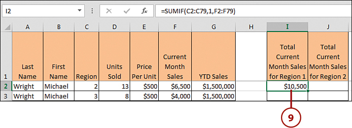
5. In the Range field, type the range of cells whose contents you want to review—for example, C2:C79. (You can also click directly in the worksheet to select the cells.)
6. In the Criteria field, type the criterion you want to check in the range—in this case, type 1 because you want to add sales data from Region 1 only.
7. In the Sum_range field, type the range of cells that match your criterion—in this case, F2:F79, which contains the current month sales data.
8. Click OK.

9. Excel adds the range given your criteria and inserts the result in the resultant cell.
Range Selection
In addition to typing specific Range and Sum_range arguments, you can click in the worksheet and select each range of cells using the mouse.
COUNTIF
Instead of totaling cells that meet a criterion with SUMIF, you can use COUNTIF to count the number of cells in a range that meet a specific criterion. For example, instead of totaling your sales data, maybe you want to know how many regional quarters were less than $20,000.
Find the Future Value of an Investment (FV)
If you open a 3 percent interest-bearing money market account with $100 in January and make deposits of $100 each month, how much money will you have at the end of the year? Excel can help you calculate the future value of an amount of money, based on a constant interest rate, over a specific number of periods in which you make a constant payment.
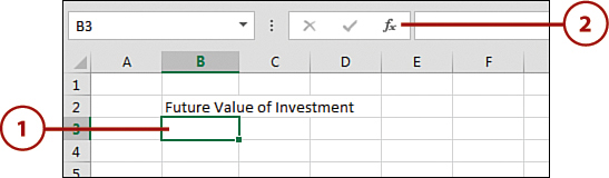
1. Click in the cell in which you want the result of the function to appear, which is called the resultant cell.
2. Click the Insert Function (fx) command next to the Formula bar.
3. The Insert Function dialog box opens. Click the down arrow next to the Or Select a Category field, and choose Financial from the list that appears.
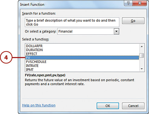
4. A list of financial-related functions appears in the Select a Function list. Scroll through the list to locate the FV function, and double-click it.
5. In the Rate field, type the interest rate per period. For example, type 3%/12 for monthly accrual on a 3 percent interest-bearing account.
6. In the Nper field, type the total number of payments for the investment (in this example, 12 deposits).
7. In the Pmt field, type the amount to be paid in each deposit—in this case, –100.
8. Click OK.

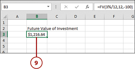
9. Excel calculates the future investment value and inserts it in the resultant cell.
Negative Payments
Because you are making a payment with each deposit, you need to make sure the Pmt argument is a negative value.
Recognizing and Fixing Errors
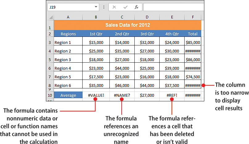
Excel notifies you when there are errors in your data by displaying different error descriptions in the cell that contains the error. For example, when a cell contains the value ####, it means that the column that contains that value is not wide enough to display the actual data. Simply widen the column to see the cell’s contents. The next few tasks explain the various types of errors and how to fix them.
1. If one of the cells in your worksheet contains the #### error, click the cell’s column border and drag it to increase the column width.

2. When you let go of the dragged border, the error disappears and the cell’s actual data is displayed.
Beginning with Larger Columns
It is a good idea to start out with columns that are larger than you need. Then you can decrease their size while you format the worksheet.
AutoFitting Column Widths
To automatically make an entire column (or multiple columns) fit the width of the widest cell in that column (or columns), move the cursor over the right side of the column header, and double-click when the cursor changes to a two-headed arrow.
Fix the #DIV/0! Error
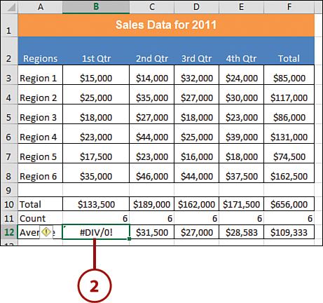
Excel notifies you when there are errors in your data by displaying different error descriptions in the cell that contains the error. For example, when a cell contains the #DIV/0! error, it means that the formula is trying to divide a number by 0, or by an empty cell.
1. In the cell you want to use as the resultant cell, type a formula to obtain an average. For example, type =SUM(B10/B9) in cell B12, and press Enter.

2. If one of the cells in your worksheet now contains the #DIV/0! error, locate the empty cell referenced by the formula (in this case, cell B9).
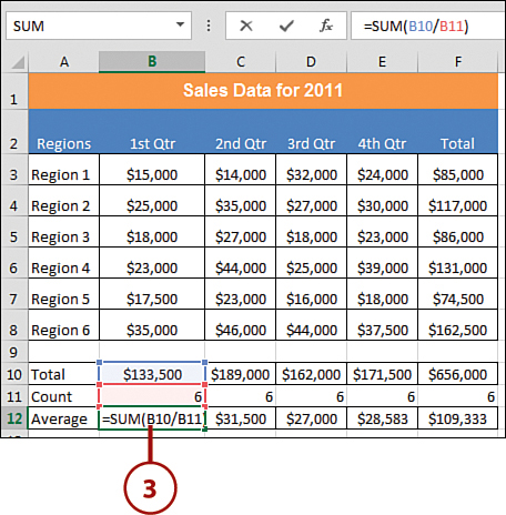
3. Click the resultant cell (here, B12), press F2 on the keyboard, and retype the formula to omit the empty cell—in this case, =(B10/B11)—and press Enter.
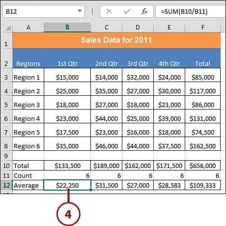
4. The error disappears because it is no longer trying to divide a number by an empty cell.
Pressing the Delete Key
In this example, you could also press the Delete key in cell B9 to remove the formula.
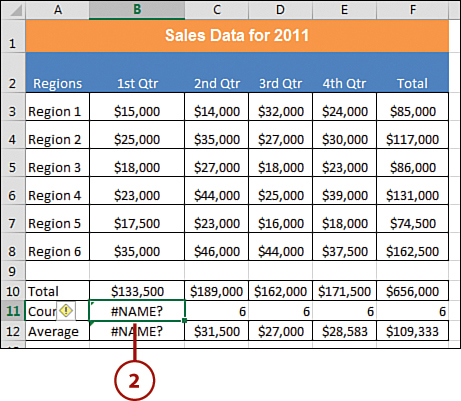
Fix the #NAME? Error
Excel notifies you when there are errors in your data by displaying different error descriptions in the cell that contains the error. For example, when a cell contains a #NAME? error, it means the formula contains an incorrectly spelled cell or function name.
1. In the cell you want to use as the resultant cell, type the formula you want to use in your calculation. For example, type =CNT(B3:B8) in cell B11, and press Enter.
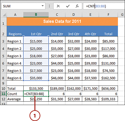
2. In this case, you get the #NAME? error because CNT is not the correct spelling for the referenced function. (It is COUNT.)
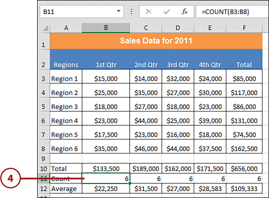
3. Click the resultant cell (here, B11), press F2 on the keyboard, and retype the formula—in this case, =COUNT(B3:B8)—and press Enter.
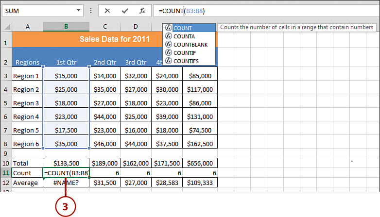
4. The error disappears because the function is spelled correctly.
Leveraging the Insert Function Dialog Box
If you are unsure about the exact syntax Excel requires for a function, consider using the Insert Function dialog box (covered earlier in this chapter in the “Finding and Using Excel Functions” section).
Fix the #VALUE! Error
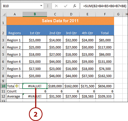
Excel notifies you when there are errors in your data by displaying different error descriptions in the cell that contains the error. For example, when a cell contains a #VALUE? error, it means the formula contains nonnumeric data or cell or function names that cannot be used in the calculation.
1. In the cell you want to use as the resultant cell, type the formula you want to use in your calculation. For example, type =SUM(B2+B4+B5+B6+B7+B8) in cell B10, and press Enter.
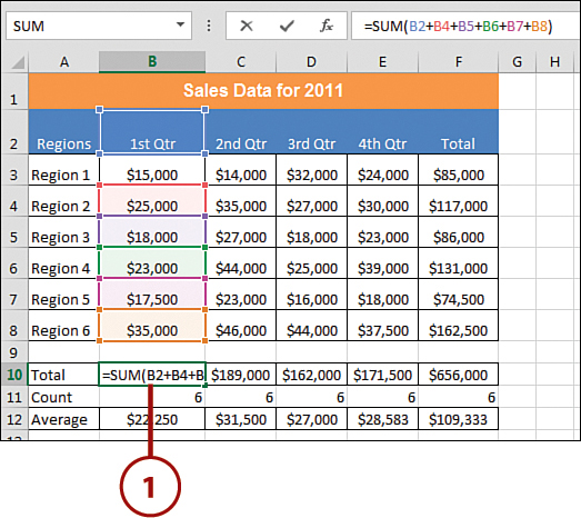
2. In this case, you get the #VALUE! error because the value in cell B2 is textual, not numeric. You won’t get the error if you either remove B2 or you replace the formula with =SUM(B2:B8) instead of the plus signs.
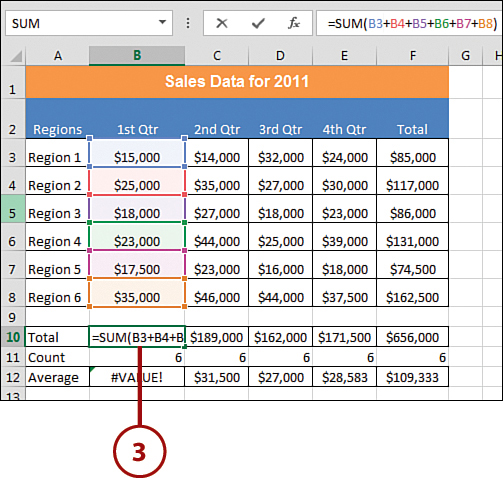
3. Click the resultant cell (here, B10), press F2 on the keyboard, and retype the formula—in this case, =SUM(B3+B4+B5+B6+B7+B8)—and press Enter.
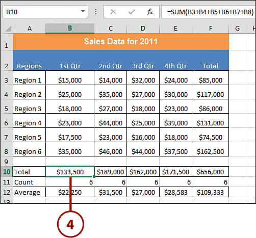
4. The error disappears because all cells are now numeric.
Overwriting Cells
See the task “Overwriting and Deleting Data” in Chapter 3, “Entering and Managing Data,” to make sure you are correctly overwriting data in cells.
Recognize the #REF! Error
Excel notifies you when there are errors in your data by displaying different error descriptions in the cell that contains the error. For example, when a cell contains a #REF! error, it means the formula contains a reference to a cell that isn’t valid. Frequently, this means you deleted a referenced cell. The best solution is to undo your action and review the cells involved in the formula.
1. In the cell you want to use as the resultant cell, type the formula you want to use in your calculation. For example, type =SUM(B2+C2+D2+E2) and press Enter.

2. Right-click one of the columns that contains a cell referenced in the formula you just typed (here, column D), and choose Delete from the shortcut menu that appears.
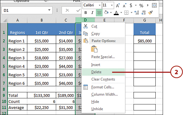
3. In this case, the #REF! error appears because the values in cells referenced in column D are no longer available in the formula.
4. Click the Undo command to correct it.

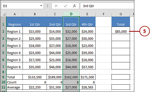
5. The error disappears because the formula values are restored.
If after you undo what caused the #REF! error you want to find out what caused it, see the tasks “Checking for Formula References (Precedents)” and “Checking for Cell References (Dependents)” later in this chapter for more information on checking formula and cell references.
Recognizing Circular References
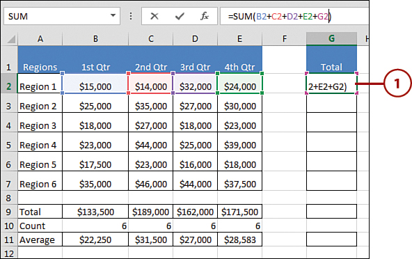
Excel notifies you when there are errors in your data by displaying different error descriptions in the cell that contains the error. For example, you receive a circular reference error message when one of the cells you are referencing in your calculation is the cell in which you want the calculation to appear.
1. Type the formula you want to use in your calculation. For example, type =SUM(B2+C2+D2+E2+G2) and press Enter.
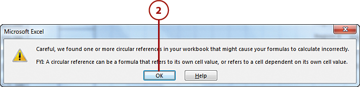
2. Excel displays an error message, notifying you that the formula contains a circular reference. Click OK.
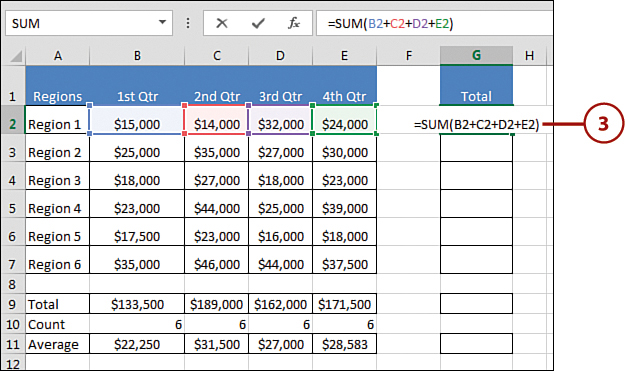
3. Click the resultant cell, press F2 on the keyboard, and edit your formula—in this case, =SUM(B2+C2+D2+E2)—and press Enter.
4. The error is fixed because the result cell no longer is in the calculation.
Circular Reference Dialog
If you didn’t intend to create a circular reference and you chose OK in the message box, the Circular Reference dialog and Help display to assist you in correcting your actions.
Checking for Formula References (PRECEDENTS)
One way to check a formula to see whether it is referencing the correct cells is to select that formula and then trace all cells referenced in that formula. Cells referenced are called precedents.
1. Click the Formulas tab.
2. Click the cell you want to trace (this cell must contain a formula) and click the Trace Precedents command.
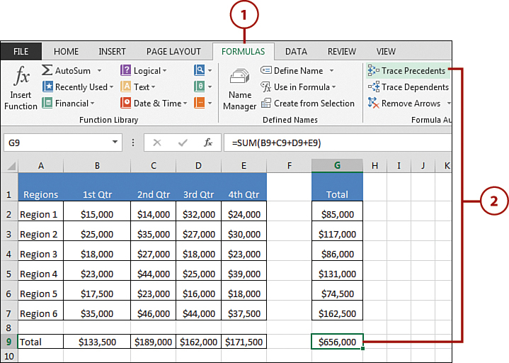
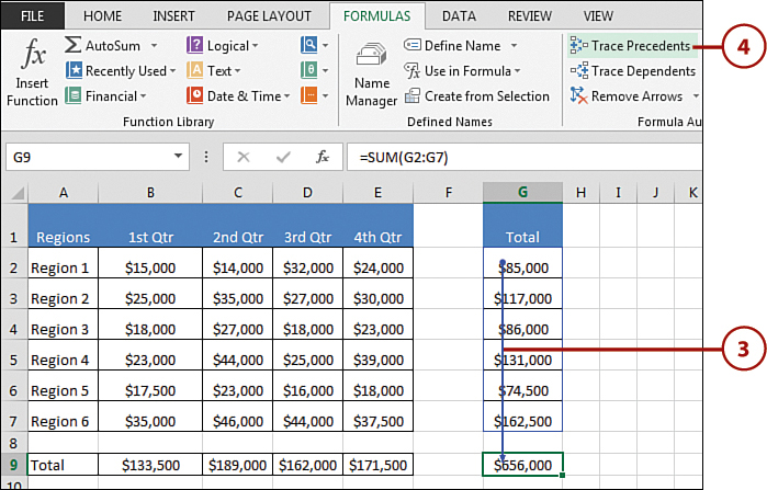
3. Excel draws tracer arrows to the appropriate cells.
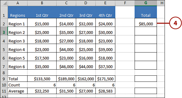
4. Click the Trace Precedents command again to see whether there are any precedents for these calculations.
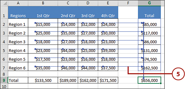
5. If additional precedents are present, Excel draws additional tracer arrows to the appropriate cells.
Removing Formula Auditing Lines References
Click the Remove Arrows command on the Formula tab to remove the arrows.
Checking for Cell References (DEPENDENTS)
When you trace a dependent, you start with a cell referenced in a formula and then trace all cells that reference this cell. This is another way to check whether your formulas are correct. (If the cell is not referenced in a formula, you get an error message saying so.)
1. Click the Formulas tab.
2. Click the cell you want to trace. This cell must not contain a formula.
3. Click the Trace Dependents command until the tracer arrows stop adding on to the appropriate cells.
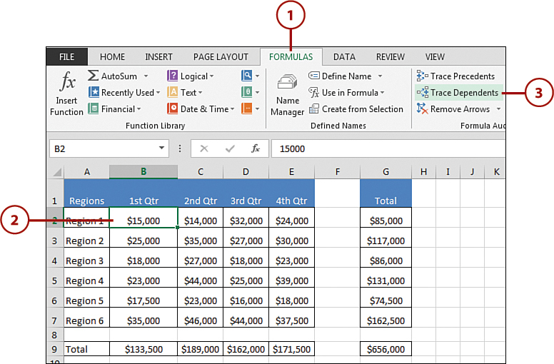
4. Excel draws tracer arrows to the appropriate cells.

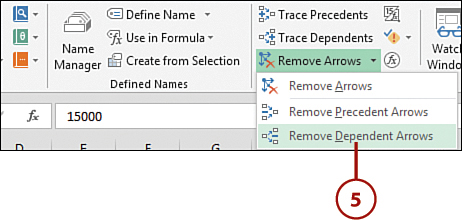
5. Click the Remove Arrows command enough times to remove all the arrows.
Using Trace Errors
If the cell contains an error message, use the Trace Errors command to have Excel trace possible reasons for the error.