
Chapter 8. A Simple Way to Describe Shape in 2D and 3D
8.1. Introduction
We now turn to a discussion of the triangle mesh, the most widely used representation of shape in graphics. Triangle meshes consist of many triangles joined along their edges to form a surface (see Figure 8.1). Other meshes, in which the basic elements are quads (quadrilaterals), or other polygons are sometimes used, but there can be problems associated with them. For instance, it’s easy to create a quadrilateral whose four vertices do not all lie in a plane; how should the interior be filled in? For triangles, this is not a problem: There’s always a plane containing any three vertices. Because triangle meshes are so widespread, we concentrate on them in this chapter.

It’s easy to see how to create certain shapes with triangle meshes. Starting with any polyhedron, for instance, we can subdivide the faces into triangles. Figure 8.2 shows this for the cube. For more complex shapes, it’s possible to approximate the shape with a mesh. One way to do this is to find the locations of many points on the shape, and then connect adjacent locations with a mesh structure. Such an approximation, if the points are close enough to one another, can look very much like a smooth surface. Consider the case of the icosahedron, which looks a lot like a sphere: Each point of the icosahedral mesh is very close to a point of the sphere, and vice versa. Similarly, each normal vector to a triangle mesh is very close to a vector normal to the sphere at a corresponding point, and vice versa. There is a distinction, however: The function that assigns normal vectors to points of the sphere is continuous, while for the icosahedron, it’s piecewise constant (the normal vector doesn’t change as you move about on a triangular facet). This distinction can be important when we try to consider the reflection of light from surfaces described with planar facets.

One of the nicest properties of triangle meshes is their uniformity. This uniformity allows us to apply various operations to them with guarantees that have relatively simple proofs; it also makes it easy to try simple ideas. Among the most interesting operations we can perform on a mesh is subdivision, in which a single triangle is replaced by several smaller triangles in a fairly simple way. (There are many subdivision algorithms, some of which we’ll discuss in Chapter 22.) Typically subdivision is used to smooth out a mesh that has sharp points or edges, so as to approach a limit surface that’s fairly smooth. Of course, repeated subdivision operations increase the triangle count substantially; this can have a major impact on rendering performance.
Another important operation on meshes is simplification, in which a mesh is replaced by another mesh that’s similar to it, topologically or geometrically, but has a more compact structure. If this is done repeatedly, one can arrive at a collection of simpler and simpler representations of the same surface, suitable for viewing at greater and greater distances. (A 10, 000-polygon object that covers only a single display pixel can almost certainly be rendered with fewer polygons, for instance—a simplified mesh is ideal here.) Hoppe [Hop96, Hop98] has studied this problem extensively.
Meshes are in common use in part because we are familiar with the geometry of triangles. Not every object in the world is well suited to mesh representation. Certain shapes, for instance, are characterized by having geometric detail at every scale (e.g., mica or fractured marble). Others have structure that is uniform in a way particularly unsuited for mesh representation, like hair, whose bent tubular structure can be far more compactly represented than with a mesh approximation.
Nonetheless, many research laboratories and commercial companies have managed to produce a great many successful images using an approach in which all shapes were approximated by triangle meshes.
8.2. “Meshes” in 2D: Polylines
The analog of a triangle mesh in space, taken one dimension lower, is a collection of line segments in the plane. (The space in which we work is one dimension lower, and the objects we’re working with are one dimension lower: line segments instead of triangles.) We’ll discuss these briefly as an introduction to mesh structures. We’ll call one of these a 1D mesh.
A 1D mesh (see Figure 8.3) consists of vertices and edges, which are line segments joining the vertices. Because the line segment between two vertices is completely determined by the vertices themselves, we can describe such a structure in two parts.
• A listing of the vertices and their locations. Typically the vertices are denoted by small integers; their locations are points in the plane.
• A listing of the edges, consisting of a collection of ordered pairs of vertices.

Figure 8.3: A 1D mesh consists of a collection of vertices and straight-line edges between them. The ones that most often interest us (shown in (a) and (b)) have one or two edges meeting each vertex, and no two edges intersect except at a vertex. But there are also meshes with more than two edges at some vertices, like (c), and ones where edges do intersect at nonvertex points (d).
The following tables describe a simple 1D mesh:

This data structure has an interesting property: The topology of the mesh (which edges meet which other edges) is encoded in the Edges table, while the geometry is encoded in the Vertices table. If you adjusted one of the entries in the Vertices table a little, the number of connected components, for instance, would not vary.
One might argue that if you moved the vertices enough, then two edges might intersect when they didn’t intersect before. That’s true, but such intersections can be removed by adjusting the vertices; the fact that the edge (1, 2) intersects the edge (2, 3) cannot be altered by moving the vertices.
Indeed, one can treat the edge table (together with a listing of the vertex indices, in case some vertex is not in any edge) as describing an abstract graph (in the sense of graph theory). From this one can compute things like the Euler characteristic, the number of components, etc.
8.2.1. Boundaries
The boundary of a 1D mesh defined as a formal sum of the vertices of the mesh in which the coefficient of each vertex is determined as follows: Each edge from vertex i to vertex j adds + 1 to the coefficient for j, and –1 to the coefficient for i; we sometimes write that the boundary of the edge ij is j – i. Applying this to the mesh above, we find that the boundary formal sum is (reading edge by edge, and writing vi for the ith vertex)
which simplifies to v6 – v5. Informally, we say that the boundary consists of vertices 5 and 6.
The reason for the formalism arises when we consider more interesting meshes, like the one shown in Figure 8.4. The boundary in this case consists of v1 + v2 + v3 + v4 + v5 – 5v0.

Figure 8.4: A wagon-wheel-shaped mesh. An arrow from vertex i to vertex j indicates that (i, j) is an edge of the mesh, and not (j, i).
A 1D mesh whose boundary is zero (i.e., the formal sum in which all coefficients are zero) has the property that it’s easy to define “inside” and “outside” by a rule like the winding number rule for polygons in the plane. Such a mesh is called closed.
A 1D mesh where each vertex has degree 2 (i.e., where each vertex has an arriving edge and a leaving edge) is said to be a manifold mesh: In the abstract graph, every point has a neighborhood (a set of all points sufficiently near it) that resembles a small part of the real number line. A point in the interior of an edge, for example, has the edge interior as such a neighborhood. A vertex has the union of the interiors of the two adjacent edges, together with the vertex itself, as such a neighborhood.
We use the term “manifold mesh” to suggest that such meshes are like manifolds, which we will not formally define; there are many books that introduce the idea of manifolds with the appropriate supporting mathematics [dC76, GP10]. Informally, however, an n-dimensional manifold is an object M with the property that for any point p ![]() M, there’s a neighborhood of p (i.e., a set of all points in M close to p, defined appropriately) that looks like the set {x
M, there’s a neighborhood of p (i.e., a set of all points in M close to p, defined appropriately) that looks like the set {x ![]() Rn : ||x|| < 1} (the “open ball”) in Rn. “Looks like” means that there’s a continuous map from the ball to the neighborhood and back. (These continuous maps are also required to be “consistent” with one another wherever their domains overlap; the precise details are beyond the scope of this book.) For example, the unit circle in the plane is a 1-manifold because one neighborhood of the point with angle coordinate θ consists of all points with coordinates θ – 0.1 to θ + 0.1; the correspondence to the unit ball in R (i.e., the open interval –1 < x < 1) is u
Rn : ||x|| < 1} (the “open ball”) in Rn. “Looks like” means that there’s a continuous map from the ball to the neighborhood and back. (These continuous maps are also required to be “consistent” with one another wherever their domains overlap; the precise details are beyond the scope of this book.) For example, the unit circle in the plane is a 1-manifold because one neighborhood of the point with angle coordinate θ consists of all points with coordinates θ – 0.1 to θ + 0.1; the correspondence to the unit ball in R (i.e., the open interval –1 < x < 1) is u ![]() 10(u – θ). Similarly, familiar smooth surfaces in 3-space like the sphere, or the surface of a donut, are 2-manifolds. An atlas (i.e., a book showing maps of the whole world) is a kind of demonstration that the sphere is a manifold: Each page of the atlas gives a correspondence between some region of the globe (e.g., Western Europe) and a portion of the plane (i.e., the page of the atlas that shows Western Europe).
10(u – θ). Similarly, familiar smooth surfaces in 3-space like the sphere, or the surface of a donut, are 2-manifolds. An atlas (i.e., a book showing maps of the whole world) is a kind of demonstration that the sphere is a manifold: Each page of the atlas gives a correspondence between some region of the globe (e.g., Western Europe) and a portion of the plane (i.e., the page of the atlas that shows Western Europe).
Shapes with corners (like a cube) can also be manifolds, but they are not smooth manifolds, which is what’s usually meant when the term is used informally—a continuous map that takes a small region around the corner of the cube and sends it to the plane ends up distorting things too much for all the required conditions for “smoothness” to hold.
Self-intersecting shapes like a figure eight in the plane fail to be manifolds, because any small neighborhood of the crossing point in the middle of the figure eight looks like a small letter “x,” which cannot be made to correspond to a unit interval in a bicontinuous way. The technicalities in defining manifolds are quite subtle (indeed, it took several decades for them to eventually settle into their modern form). Fortunately for us, the shapes we use in graphics are generally “polyhedral manifolds.” The definitions are still subtle, but there are key theorems that tell us that in the one- and two-dimensional cases, we can instead verify that something’s a manifold by using far simpler methods. Those simpler methods are precisely the content of our notions of a manifold vertex-and-edge mesh, and a manifold triangle mesh (which we’ll define shortly).
Your goal, in reading the definitions here, should not be to gain a deep understanding that you could use to prove theorems—that requires a much more thorough treatment. But you should, when done, be able to say, “Sure, I can look at a simple mesh and identify it as a manifold mesh, or perhaps manifold-with-boundary mesh.”
Manifold meshes are commonplace and particularly easy to work with (and to prove theorems about). Note that the definition does not say that a manifold mesh must have only one connected component; indeed, a mesh consisting of two nonintersecting triangles is a valid manifold mesh. So is the empty mesh.
The meshes we’ve described, in which each edge is an ordered pair, are called oriented meshes; if we had described edges by unordered pairs, we would have had an unoriented mesh, in which case the definition of “boundary” would have made no sense. We’ll have no further use for such meshes, however.
8.2.2. A Data Structure for 1D Meshes
To prepare for the discussion of 2D meshes in 3-space, we’ll describe a data structure for 1D meshes in 2-space first, one which has strong analogies with more complex structures. The components are
• A vertex table, consisting of vertex indices and the associated points in the plane
• An edge table, consisting of ordered pairs of edges
• A neighbor-list table, consisting of an ordered cyclic list of edges meeting a vertex so that one can read off the list of edges at a vertex (in counterclockwise order)
We already encountered such a structure when we discussed subdivision of curves (see Figure 8.5) in Chapter 4.

Figure 8.5: The square at left is subdivided to become the octagon at right. Note that for each vertex of the square, there’s a vertex in the octagon, and for each edge of the square, its midpoint is a vertex of the octagon as well.
The operations supported by this data structure (and their implementations) are as follows.
• Insert a vertex: Add it to the vertex table; leave other tables untouched.
• Insert an edge (i, j): Add it to the vertex table and the edge table (both O(1)); add it to the neighbor-list table both at vertex i and at vertex j. Insertion in the neighbor list for vertex i can take O(e) time, where e is the number of edges in the table (one must insert it in the right place in the counterclockwise ordering of edges around vertex i, which might contain all e edges). In a manifold mesh, however, where there can be, at most, two edges at a vertex, this operation is O(1).
• Get the edges meeting vertex i. (This is O(1), since it consists of the neighbor list for vertex i.)
• Given a vertex i and an edge e containing i, find the other end of e.
• Given an edge e, find its two endpoints.
• Delete an edge. This requires deletion from the edge table, and if the edge is (i, j), deleting the edge from the neighbor lists for i and j, which may be an O(e) operation, but in the manifold case is O(1).
The choice of how to implement the vertex and edge tables depends on the expected use. An array implementation is convenient if there will be no deletions. But if there will be deletions, one must do one of the following.
• Mark array entries as invalid somehow.
• Shift the array contents to “fill in” when an item is deleted (which requires updating indices stored in other tables).
The marked-entries approach can create large but mostly empty tables if there are many insertions and deletions so that the “list all vertices” or “list all edges” operations become slow. The content-shifting approach actually works quite well, however. To start with a simple case, if there are n vertices and we want to delete vertex n, we just declare the end of the array to be the n – 1st element, and delete all references to vertex n in other tables. To delete a different vertex—say, the second one—we reduce the problem to the earlier case: We exchange the second and the nth vertices, and then delete the nth. This requires replacing all references to vertex index 2 with vertex index n, and vice versa, in the other tables, but that’s fairly straightforward.
Note that the choice to store the edges that meet a vertex is also application-dependent. It makes finding all vertices of topological distance one from vertex i very fast, but at the cost of making edge addition somewhat slow in the worst case. If you do not anticipate needing to find the neighbors of vertex i, maintaining a neighbor list is pointless. Similarly, the choice to store the neighbor lists in a counterclockwise-sorted order is useful primarily if one is interested not only in the structure of the 1D mesh, but also in the structure of the 2D regions into which it divides the plane; if these are of no interest, then the neighbor lists can be stored in hash tables or other similarly efficient structures (or in a two-element array, in the case of manifold meshes).
8.3. Meshes in 3D
The situation in 3D is analogous to that in 2D: To describe a mesh, we list the vertices and the triangles of the mesh. What about the edges? The tradition in graphics has been to infer the edges from the triangles: If vertices i, j, and k form a triangle, then the edges (i, j), (j, k), and (k, i) are assumed to be part of the mesh structure. This means that one cannot have dangling edges (see Figure 8.6), although isolated vertices are still allowed. The general descriptions of mesh structures (consisting of vertices, edges, triangles, tetrahedra, etc., with coordinates associated only to the vertices, and then extended to higher-dimensional pieces by interpolation) have been at the foundation of topology for more than 100 years [Spa66]; the student interested in such structures should consult the topology literature to avoid reinventing things.

Figure 8.6: A triangle with a dangling edge, like the one shown here, cannot be represented by our mesh structure.
In graphics, however, the structure of a vertex table and “face table” or “triangle table” is well established. As in the 1D case, insertion of vertices and triangles is fast, and deletion of vertices is slow (because all associated triangles must be found and deleted). If we store a neighbor list for each vertex, deletion becomes faster. Because the neighbor list of triangles meeting a vertex is unordered, the insertion cost is low, but the deletion cost is high. When additional constraints are imposed on the mesh, the triangle list for a vertex can be ordered, slightly increasing insertion and deletion costs, but simplifying other operations like finding the two faces adjacent to an edge.
What about edges? While we cannot insert an edge, we can ask questions like “Is this pair of vertices an edge of the mesh?” In other words, is it the edge of some triangle of the mesh? And given a triangle with vertices i, j, and k, we can ask, “What are the other triangles that contain the edge (i, j)? These questions are O(T), in the sense that answering them requires an exhaustive search of the triangle list. In special cases, which we discuss in the next section, they can be made faster.
If you are eager, at this point, to get on with making objects and pictures of objects, you can safely skip the remainder of this chapter and use the vertex- and triangle-table structure for meshes until you encounter problems with space or efficiency, at which point the remaining sections will be of use to you. If, on the other hand, you’d like to know more about how to work with meshes effectively, read on.
8.3.1. Manifold Meshes
A finite 2D mesh is a manifold mesh if the edges and triangles meeting a vertex v can be arranged in a cyclic order t1, e1, t2, e2, ..., tn, en without repetitions such that edge ei is an edge of triangles ti and ti+1 (indices taken mod n). This implies that for each edge, there are exactly two faces that contain it.
We can store a manifold mesh in a data structure analogous to the one we described for 1D meshes, consisting of a vertex table, a triangle table, and a neighbor-list table.
The neighbor list for vertex i consists of the triangles surrounding vertex i, in some cyclic order (so the kth and k + 1st triangles in the list share an edge). (One can no longer disambiguate between the two possible cyclic orderings around a vertex with a notion like “counterclockwise,” unfortunately, unless the manifold is oriented, which we describe in the next section.)
Manifold meshes unfortunately don’t admit insertions or deletions of triangles: Any insertion or deletion ruins the manifold property. But it is easy to find the vertices adjacent to a given vertex (i.e., given a vertex index i, we can find all vertex indices j such that (i, j) is an edge): We simply take the set of all vertices of all triangles in the neighbor list for vertex i, and then remove vertex i.
It’s also fairly easy, given a triangle containing edge (i, j), to find the other triangle containing that edge.
8.3.1.1. Orientation
We’ll often have reason to care about the orientation of triangles in a mesh (see Figure 8.7) so that the triangles (1, 2, 3) and (2, 1, 3) are considered different (the triples are listings of vertex indices). One use of an orientation is in the determination of a normal vector: If the vertices of a nondegenerate triangle (i.e., one with a nonzero area) are at locations Pi, Pj, and Pk, then we can compute (Pj – Pi) × (Pk – Pi), which is a vector perpendicular to the plane of the triangle.1 Note that if we exchange vertices Pj and Pk, the resultant vector is negated. Since we often use the normal to a triangle in a mesh to determine what’s “inside” or “outside” the mesh, the ordering of the vertices is critical.
1. The description of the cross product and further discussion of normal vectors was given in Chapter 7.

Figure 8.7: Two adjacent triangles in a mesh with consistent normal vectors (i.e., the normal vector tips are on the “same side” of the mesh). Note that the edge (i, j) is an edge of one triangle, but (j, i) is an edge of the other. In general, in a consistently oriented mesh, each edge appears twice, in opposite directions.
If two adjacent triangles (see Figure 8.8) have consistently oriented normal vectors, then the edge they share will appear as (i, j) in one triangle and as (j, i) in the other. And if a manifold mesh can have its triangles oriented so that this is true, it can also be given consistently oriented normal vectors. This is a nontrivial theorem from combinatorial topology.
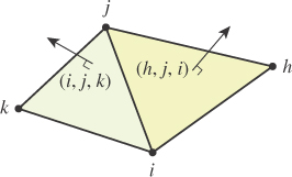
Figure 8.8: The triangles of this mesh are oriented; the circular arrows indicate the cyclic ordering of the vertices. Note that the vertex triples (1, 2, 3) and (2, 3, 1) indicate the same oriented triangle (i.e., there are three equivalent descriptions of every oriented triangle).
When a manifold is oriented, the triangles around a vertex have a natural order. Suppose that surrounding vertex 1 there are the triangles (5, 1, 2), (4, 3, 1), (1, 5, 4), and (1, 3, 2). We can cyclically permute each to put vertex 1 first: (1, 2, 5), (1, 4, 3), (1, 5, 4), and (1, 3, 2). Now starting with the first triangle, we can consider its “first” and “last” edges, (1, 2) and (5, 1). We choose, as our next triangle, the one whose first edge is the opposite, (1, 5), of this last edge. That’s (1, 5, 4). And the last edge of (1, 5, 4) is (4, 1); (1, 4) is the first edge of (1, 4, 3), whose last edge is (3, 1); (1, 3) is the first edge of (1, 3, 2), and we’ve ordered the triangles: (1, 2, 5), (1, 5, 4), (1, 4, 3), (1, 3, 2).
8.3.1.2. Boundaries
More interesting than manifold meshes (and more common as well) are meshes whose vertices are manifold or boundarylike (see Figure 8.9), in the sense that instead of the adjacent triangles forming a cycle, they form a chain, whose first and last elements share only one of their edges with other triangles in the chain; the other edge of the first triangle that meets the vertex is contained only in the first triangle, and not in any other triangle of the mesh. (The same condition applies to the last triangle.) This unshared edge is called a boundary edge, and the vertex is called a boundary vertex. Vertices that are not boundary vertices are called interior vertices.

Figure 8.9: (left) A manifold vertex has a cycle of triangles around it; (right) by contrast, a boundarylike vertex v has a chain of triangles around it—the starting and ending triangles of the chain each share only one of their edges with other triangles of the chain. The other edges of those triangles that contain v are boundary edges.
8.3.1.3. Boundaries and Oriented 2D Meshes
Just as we defined the boundary of an edge from vertex i to vertex j to be the formal sum vj – vi, we can define the boundary of a triangle in a mesh with vertices i, j, and k to consist of the formal sum of edges
Furthermore, we can define an algebra on these formal sums in which the vertex (i, j) is identified with –1(j, i) so that the boundary above could be written
instead. We can define the boundary of a collection of oriented triangles as the formal sum of their boundaries.
For an oriented manifold mesh, this boundary will be zero (i.e., the coefficient of each edge will be zero), because if (i, j) is part of the boundary of one face, then (j, i) = –(i, j) is part of the boundary of another.
For an oriented manifold-with-boundary mesh, the boundary will consist of exactly the edges we identified above as “boundary edges.” In general, an oriented mesh with no boundary edges is called closed.
8.3.1.4. Operations on Manifold-with-Boundary Meshes
Manifold-with-boundary meshes support operations like vertex and face insertion and deletion. The efficiency of each operation depends on the implementation. If the representation is simply vertex tables and face tables, then insertion is O(1), and deletion (after the “exchange with the last item in the list” trick) is too. If we maintain a neighbor list for each vertex, then insertion becomes O(T), where T is the number of triangles, as does deletion.
Note that computing the boundary of such a mesh can be done in O(T) time. (Use a hash table to count the number of times each edge appears, with sign. If the edge appears zero times, delete it from the hash table.) But one can also maintain a record of the boundary during insertions and deletions so that reporting it at any time is an O(1) operation.
8.3.2. Nonmanifold Meshes
Just as in the 1D case, we sometimes encounter shapes that are not well represented by manifolds or manifolds with boundary. The two cubes shown in Figure 8.10 share a vertex which is a nonmanifold vertex; two cubes sharing an edge are similarly nonmanifold. There is an important difference between the two cases, however: It’s easy to encounter a nonmanifold vertex in the course of constructing a manifold with boundary (see Figure 8.11). But once we construct a nonmanifold edge (one with three or more faces meeting it), it can never become a manifold edge through further additions.
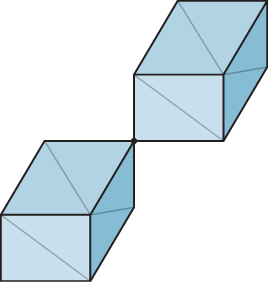

Figure 8.11: The pyramid at left has six faces; the bottom square is divided into two triangles that you cannot see. If we construct the pyramid so that after four triangles have been added, it appears as shown at the right, then the apex vertex is neither an interior vertex nor a boundary vertex according to the definitions, so this shape is neither a manifold nor a manifold with boundary. Once we add another face, it becomes a manifold with boundary, and when we add the last face, it becomes a manifold.
Each vertex in the directed-edge structure also contains a reference to one of the edges containing it (see Figure 8.12). This allows one to compute the neighborhood of the vertex (all edges and triangles that meet it) in time proportional to the size of the neighborhood.
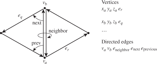
Figure 8.12: The directed-edge data structure (following Figures 4 and 5 of [CKS98]). A directed edge stores a reference to its starting and ending vertex, to the previous and next edges, and to its neighbor. For each real edge of the mesh, there are two directed edges, in opposite directions. Each vertex stores its coordinates and a reference to one of the directed edges that leaves it.
Campagna et al. [CKS98] show how this structure can be extended to handle non-manifold vertices and edges, and how to trade time for space by simplifying the structure for very large meshes.
For more general planar meshes, in which the faces may not be triangles, one can use the winged-edge data structure [Bau72], which associates to each edge of the mesh the next edge of the face to its right, the next edge of the face to its left, and the previous edges of each of these as well (see Figure 8.13). This suffices to recover all the faces and edges, provided that all faces are simply connected (i.e., no face has a ringlike shape, like the surface of a moat). The winged-edge structure also stores, for each vertex, its xyz-coordinates, and a reference to one of the edges that it lies on (from which one can find all other edges). For each face, the structure stores a reference to one edge of the face (from which one can find all the others).

Figure 8.13: The winged-edge data structure records a “previous” and “next” pointer for the faces on each side of each edge.
8.3.3. Memory Requirements for Mesh Structures
Each of the structures we’ve described for representing meshes has certain memory requirements. Assuming 4-byte floating-point representations and 4-byte integers, we can compare their memory requirements as done by Campagna et al. [CKS98].
The vertex-table-and-triangle-table approach takes 12V bytes for the V vertices and 12T bytes for the T triangles. How are the number of vertices and triangles related? For a mesh representing a closed surface, Euler’s formula tells us that V – E + T = 2 – 2g, where g is the genus of the surface.2 Assuming further that every vertex is actually part of some triangle (so that the vertex table does not contain lots of unused vertices), and that the mesh is closed, we can simplify this: Each triangle has three edges, and each edge is shared by two triangles. So the number of edges, E, is ![]() . Thus,
. Thus,
2. The genus of a closed surface is, informally, the number of holes in it. A sphere has genus zero, a torus has genus one, a two-holed torus has genus two, etc. A slice of Swiss cheese tends to have quite high genus.
which simplifies to
For low-genus surfaces with fine tessellations, the right-hand side is negligible compared to the left, so we find that the number of triangles is approximately twice the number of vertices; this gets us a total of 12(T + V) ≈ 12(3V) = 36V ≈ 18T bytes of storage. For the remaining mesh representations, we’ll assume that we’re representing closed manifolds of low genus so that we can replace V with ![]() and vice versa.
and vice versa.
For the winged-edge structure, each vertex uses 16 bytes (three floats and an edge reference); each face uses four bytes (one edge reference), and each edge has four edge references, two face references, and two vertex references, for a total of eight references or 32 bytes. The total, again assuming we use triangular faces only, is 16V + 32E + 4T ≈ 8T + 32![]() + 4T = 60T.
+ 4T = 60T.
For the directed-edge data structure (in the store-all-references form), each vertex uses 12 bytes for coordinates and four for an edge reference. Each directed edge contains references to two vertices and three edges, using 20 bytes. Triangular faces are not explicitly represented. So the memory use is
bytes. Note that in the analysis above, we assumed that a vertex or edge reference required only four bytes; for more complex meshes, this byte count may have to be increased in proportion to ![]() .
.
8.3.4. A Few Mesh Operations
One of the advantages of triangle meshes is that their homogeneity makes certain operations easy to perform. For manifold meshes, the homogeneity is even greater. In mesh simplification, for instance, one of the standard operations is an edge collapse, in which one edge is shrunk until it has length zero, resulting in the two adjacent triangles disappearing. In mesh beautification (where we try to make a mesh have nearly equilateral triangles and other nice properties), the edge-swap operation helps turn two long and skinny triangles into two more nearly equilateral ones. Both involve minimal operations on the data structure itself.
8.3.5. Edge Collapse
In the edge-collapse operation (see Figure 8.14), a single edge of a mesh is removed [HDD+93]. The two triangles that contain this edge are both eliminated, and the other two edges of each of them become a single edge in the new mesh. The vertices at the end of the eliminated segment become a single vertex.

Figure 8.14: The edge from vertex va to vertex vb is collapsed; the edge itself and the two adjacent faces are removed from the data structure; and the other two edges of the upper face, drawn in blue, become one, as do the two edges of the lower face, drawn in red. Nothing else changes. The two vertices va and vb become a single vertex.
The description above is purely topological; there’s a geometric question as well: When we merge the two vertices, we must choose a location for the merged vertex. The location we choose depends on the goal of our simplification (see Figure 8.15). If computation is at a premium, simply using one of the old vertices as the new one is very fast. If we want to preserve some sort of shape, averaging the two vertices is easy. If such an averaging process moves a lot of points, and this will be visually distracting, we can choose a new location that minimizes the average or extreme distance between the old and new meshes. There is no one “right answer.” As in most of graphics, the choice you make depends on your intended use of the data structure.

Figure 8.15: Different geometric choices for an edge collapse in 2D. The edge AB is collapsed; one can (a) place the collapsed vertex at A for computational simplicity, (b) at the midpoint of the segment AB, or (c) at a point Q that minimizes the maximum (or average) distance from every old mesh point to the nearest new mesh point. Other goals are possible as well.
8.3.6. Edge Swap
Meshes that get distorted or deformed in the course of an application’s use of them may eventually get so deformed that individual triangles are long and skinny. Such triangles are characterized by their bad aspect ratios. In general, one can define an aspect ratio for a planar shape (see Figure 8.16) by finding, among all rectangles that enclose the object and touch it on all four sides (these are called bounding boxes), the one whose length-to-width ratio is greatest. This ratio is then called the aspect ratio. High-aspect-ratio triangles produce bad artifacts in many situations, so it’s nice to be able to eliminate them when possible. An edge-swap operation (see Figure 8.17) can convert two adjacent high-aspect-ratio triangles to two with lower aspect ratios. (It can also, done in reverse, do the opposite: Selecting the right edge to swap in order to beautify a mesh requires examining the impact of each possible swap.)

Figure 8.16: The aspect ratio of a planar shape is determined by finding the bounding box for the object for which the ratio of length to width is greatest.

Figure 8.17: The triangles adjacent to the edge from va to vb both have bad aspect ratios. By replacing the edge vavb with the edge vcvd, we get a new pair of triangles whose aspect ratios are better.
Notice that the swap removes two triangles from the mesh structure and replaces them with two others. In the simple vertex- and triangle-table structure, this operation is trivial. In the directed-edge structure, the implementation is more complex, because (a) some vertex may point to the edge that’s being swapped out, and this edge pointer needs to be found and replaced; and (b) it makes sense to replace the two old triangles with the two new ones, but there’s substantial shuffling of directed edges in this process, and making sure that the new directed edges point to the correct new triangles is messy.
8.4. Discussion and Further Reading
Triangle mesh representations and other representations for nontriangle meshes, for planar graphs, and for simplicial complices—assemblies of vertices, edges, triangles, tetrahedra, etc.—are widely studied in areas other than graphics; each representation is tuned to the application area. We’ve described a few representations here that are particularly suited to work in graphics, but those who develop CAD programs, for instance, may have to deal with computing the union and intersections of shapes represented by meshes. Unfortunately, the union of two manifold meshes (e.g., two cubes) may not be a manifold mesh (if the cubes share just one vertex, or just one edge), so structures suitable for nonmanifold representations may be essential. Those working in finite-element modeling of mechanical structures or fluid flow have their own constraints, such as the need for triangles and tetrahedra to be nicely shaped (no small angles in any triangles), or to have their size vary depending on the region in which they lie (e.g., turbulent flow may require a fine triangulation, while smooth flow may be adequately represented by a coarse one).
For most elementary graphics, the vertex- and triangle-table representations are adequate; their incredible simplicity makes them very versatile, and if you’re implementing your own mesh structures, they’re very easy to program properly. As your needs evolve, more complex structures may be suitable; be certain that you evaluate the more complex structures to ensure that their complexity solves your particular problem.
One structure we’ve completely ignored is the “list each triangle separately as a triple of xyz-coordinates structure.” Although this is simple, it has so many disadvantages that we can never recommend its use. In particular, the only way to tell whether two triangles or edges share a vertex is with floating-point comparisons: If you move one copy of a vertex, you must move all others if you want to preserve the adjacency structure of the mesh; and determining any sort of adjacency information is, in general, O(T).
8.5. Exercises
Exercise 8.1: Suppose you know that triangle (i, j, k) is one of the triangles of a manifold mesh that’s represented by a vertex table and a face table. Then edge (i, j) is in the mesh. Describe how to find the other triangle containing edge (i, j). Express the running time of this operation in terms of T, the number of triangles in the mesh. Draw an exemplar class of meshes that shows that the upper bound you found is actually realized in practice.
Exercise 8.2: Implement a form of the 1D mesh structure that’s suitable for implementing a subdivision operation on manifold meshes. Given such a mesh, M, the associated subdivision mesh M′ has one vertex for each vertex v of M: If the neighbors of v are u and w, the new vertex is at location ![]() . M′ also has one vertex for each edge of M: If the edge is between vertices t and u, the associated vertex of M′ is at
. M′ also has one vertex for each edge of M: If the edge is between vertices t and u, the associated vertex of M′ is at ![]() . Vertices in M′ are connected by an edge if their associated vertices and/or edges in M meet (i.e., the vertex associated to the edge from u to v is connected to the vertex associated to u and to the vertex associated to v). Figure 8.5 shows an example. The parameter α determines the nature of the subdivision. The example shown in the figure uses α = 0.5; on repeated subdivision, the square becomes a smoother and smoother curve. What happens for other values of α? Use the standard 2D test bed to make a program with which you can experiment. Note: Not every manifold mesh has just a single connected component.
. Vertices in M′ are connected by an edge if their associated vertices and/or edges in M meet (i.e., the vertex associated to the edge from u to v is connected to the vertex associated to u and to the vertex associated to v). Figure 8.5 shows an example. The parameter α determines the nature of the subdivision. The example shown in the figure uses α = 0.5; on repeated subdivision, the square becomes a smoother and smoother curve. What happens for other values of α? Use the standard 2D test bed to make a program with which you can experiment. Note: Not every manifold mesh has just a single connected component.
Exercise 8.3: Explain why, in a manifold surface mesh, each vertex must have at least three adjacent triangles.
Exercise 8.4: Write pseudocode explaining how, given a vertex reference in a directed-edge data structure, to determine the list of all directed edges leaving that vertex in time proportional to the output size.
Exercise 8.5: Explain, in pseudocode, how, given a reference to a face in the winged-edge data structure, one can find all the edges of the face.
Exercise 8.6: Suppose that M is a connected manifold mesh with no boundary. M may be orientable without being oriented: It’s possible that there’s a consistent orientation of the faces of M, but that some faces are oriented inconsistently.
(a) Assuming that M is connected, describe an algorithm, based on depth-first search, for determining whether M is orientable.
(b) If M is orientable, explain why there are, at most, two possible orientations. Hint: Your algorithm may show why, once a single triangle orientation is chosen, all other triangle orientations are determined.
(c) If M is orientable, explain why there are exactly two orientations of M.
(d) Now suppose that M is not connected, but has k ≥ 2 components. How many orientations of M are there?
Exercise 8.7: The 2D test bed was designed to aid in the study of things like meshes. Use it to build a program for drawing polylines in a 2D plane, getting mouse clicks, and reporting the closest vertex to a click (perhaps by changing the color of the vertex).
Exercise 8.8: Add a feature so that a shift-click on a vertex initializes edge drawing: The starting vertex is highlighted, and the next vertex clicked is connected to the starting vertex with an edge; if there’s already an edge between the two, it should be deleted. And if the next click is not on a vertex, a vertex is created there and an edge from the preselected vertex to the new one is added. Modify the program to handle 2D meshes (i.e., vertices and triangles) by allowing the user to control-click on three vertices to create a triangle (or delete it if it already exists).