8. Filtering and Consolidating Data

This chapter shows you how to use Excel’s filtering functionality to look at just the desired records. It also shows you how to create a list of unique items, delete duplicates, and consolidate data.

Filtering and consolidating data are important tools in Excel, especially when you are dealing with large amounts of data. The filtering tools can quickly reduce the data to the specific records you need to concentrate on. The consolidation tool can bring together information spread between multiple sheets or workbooks.

Preparing Data

To make the most out of Excel’s filtering capabilities, your data should adhere to a few basic formatting guidelines:

• There should be no blank rows or columns. The occasional blank cell is acceptable.

• There should be a header above every column.

• Headers should be in only one row.

If these guidelines aren’t followed, Excel can get confused and is unable to find the entire table or header row on its own. Also, Excel can only work with one header row—any rows after the first header row get treated like data.

Applying a Filter to a Data Set

Filtering allows you to view only the data you want to see by hiding the other data. You can apply a filter to multiple columns, narrowing down the data. As you filter the data and rows are hidden, the row headers (1, 2, 3, etc.) become blue. Anytime you see blue row headers, you know the data has been filtered. An icon that looks like a funnel will replace the arrow on the column headings that have a filter applied, as shown in the Customer heading in Figure 8.1.

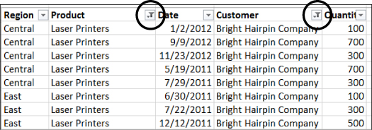
Figure 8.1. You can tell which column(s) are filtered by the filter icon where the drop-down arrow used to be.

The Filter button is a toggle button. Click it once to turn filtering on and click it again to turn filtering off. To activate the filtering option, select a single cell in the data set and use one of the following:

• On the Home tab, select Editing, Sort & Filter, Filter.

• On the Data tab, select Sort & Filter, Filter.

• When a data set is turned into a Table (Insert, Tables, Table), the headers automatically become filter headers.

When a filter is applied to a data set, drop-down arrows appear in the column headers. Click on an arrow to open up the Filter dialog box, which remains open until you click OK, Cancel, or click outside the dialog box. One or more selections can be made from each drop-down, filtering the data below the headers. Filters are additive, which means that each time a filter selection is made, it works with the previous selection to further filter the data.

Clearing a Filter

A filter can be cleared from a specific column or for the entire data set. To clear all the filters applied to a data set, use one of the following methods:

• On the Home tab, select Editing, Sort & Filter, Clear.

• On the Data tab, select Sort & Filter, Clear.

• Turn off the filter entirely using one of the following methods:

• On the Home tab, select Editing, Sort & Filter, Filter.

• On the Data tab, select Sort & Filter, Filter.

To clear all the filters applied to a specific column, use one of the following methods:

• Click the filter drop-down arrow and select Clear Filter from Column Header.

• Click the filter drop-down arrow and select Select All from the filtering list.

• Right-click a cell in the column to clear and select Filter, Clear Filter from Column Header.

Reapplying a Filter

If data is added to a filtered range, Excel does not automatically update the view to hide any new rows that don’t fit the filter settings. You can refresh the filter’s settings so they include the new rows through one of the following methods:

• On the Home tab, select Editing, Sort & Filter, Reapply.

• On the Data tab, select Sort & Filter, Reapply.

• Right-click a cell in the filtered data set and select Filter, Reapply.

Turning Filtering On for One Column

Filtering can be turned on for a single column or for two or more adjacent columns. Even though you can only select a filter item in select columns, the filter is applied to the entire table. This can be useful if you want to limit the filtering users can apply. If the sheet is then protected, users cannot turn on filtering for the other columns (see “Allowing Filtering on a Protected Sheet” for more information).

To control what column has filtering, select the header and the first cell directly beneath the header. Then do one of the following:

• On the Home tab, select Editing, Sort & Filter, Filter.

• On the Data tab, select Sort & Filter, Filter.

Filtering for Listed Items

The filter listing, shown in Figure 8.2, is probably the most obvious filter tool when you open the drop-down. For text, numbers, and ungrouped dates, a listing of all unique items in the column appears (see the “Filtering the Grouped Dates Listing” section if dates appear grouped by year and month). All items will be checked because they are all visible the first time you open the drop-down, but you can select just the items that should appear in the data. Any item that no longer bears a check mark will be hidden.

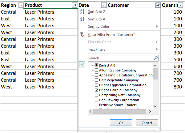
Figure 8.2. Filter a column by selecting the item(s) you want to see from the dialog box.

We have a table of the sales of various printers in 2011 and 2012. We want to narrow the table down to Laser Printers sold to Bright Hairpin Company. To filter columns for specific items, follow these steps (if filtering a Table [Insert, Tables, Table], skip to step 3):

1. Select a single cell in the data set to apply filtering to.

2. Go to Data, Sort & Filter, Filter.

3. Open the drop-down of the Product column.

4. Unselect the Select All item to clear all the check marks in the list.

5. Select Laser Printers and click OK. Now only Laser Printers are shown in the table.

6. Repeat steps 3–5 for the Customer column and Bright Hairpin Company.

7. Click OK. The sheet will update, showing only the items selected.

Filtering the Grouped Dates Listing

Dates in the filter listing are grouped by year, month, and day. All items will be checked because they are all visible the first time you open the drop-down, but you can select just the items that should appear in the data. Any item that no longer bears a check mark will be hidden.

If you click the + icon by a year, it opens up, showing the months. Click the + icon by a month and it opens up to show the days of the month. An entire year or month can be selected or unselected by clicking the desired year or month. For example, to deselect 2011 and January 2012 in Figure 8.3, deselect the 2011 group, and then deselect the January group under 2012. The data filters to show only February through December 2012.

To filter for only June 12–14, 2012, follow these steps (if filtering an existing Table, skip to step 3):

1. Select a single cell in the data set to apply filtering to.

2. Go to Data, Sort & Filter, Filter. Click OK to continue.

3. Open the drop-down of the Date column to filter.

4. Deselect the Select All item to clear all the check marks in the list.

5. Click the + icon to the left of 2012.

6. Click the + icon to the left of June.

7. Select 12, 13, and 14.

8. Click OK. The sheet updates, showing only the dates selected.

Using the Search Function to Filter for or Exclude Items

If you have a long list of items in the filter listing, you can do a search for items to include or exclude from the filter. Searches are done on the entire data list, not just the items currently filtered on. Use an asterisk (*) as a wildcard for one or more characters before, after, or in between any of the search terms.

When a search term is entered in the Search field, the filter listing below the field updates with all matches selected. You can deselect the items you want to exclude from the filter, check Add Current Selection to Filter if you do not want to lose any items you previously filtered for, and click OK.

You should keep the following in mind when using the Search function:

• The search looks through the entire column, including items you may have already filtered out.

• The Search function is additive when the Add Current Selection to Filter is selected. If not selected, each search’s results are treated as a new filter.

• To exclude items from the listing, deselect them from the result.

Column A of Figure 8.4 is a list of various television models. I want to narrow the list to just Samsung, non-LED models. To perform the two filters, follow these steps:

1. Open the filter drop-down.

2. In the Search field, type Samsung.

3. Click OK. The list on the sheet filters to just the Samsung models.

4. Open the filter drop-down again.

5. In the Search field, type LED.

6. Because I actually want all types except LEDs, deselect Select All Search Results.

7. Because I want to retain my previous Samsung results, select Add Current Selection to Filter.

8. Click OK. The list filters to all non-LED Samsung TVs, as shown in Figure 8.4.

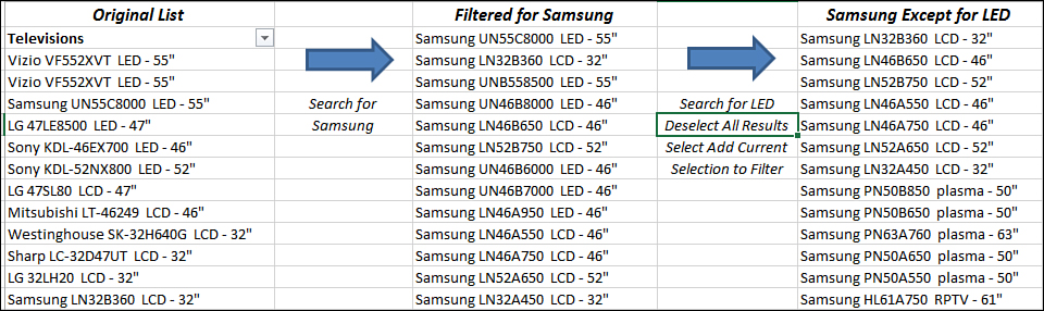
Figure 8.4. The Search function can be used to narrow down items to include in or exclude from the filter.

Using the Search Function on Grouped Dates

If you have a lot of dates in the filter listing, you can search for specific years, months, or dates to include or exclude from the filter. Searches are done on the entire data list, not just the items currently filtered on.

The Search function for grouped dates includes a drop-down, shown in Figure 8.5, allowing you to search by year, month, or date. The Search drop-down has the following options:

• Year—Search results are grouped by year.

• Month—Search results are grouped by year and then month. The search term must be the long version of the month, such as January.

• Date—Search results are grouped by year, then month, then day. Because the search will return partial matches, you should use the two-digit variation for dates. For example, to search for the 1st of a month, enter 01 instead of 1. If you enter 1, every date with a 1, such as 10, 11, 12, will be returned.

• All—Search results are grouped by year, then month, then day. This option looks for a match anywhere in the date. For example, if your data set includes dates from 2009 and the search term is 09, all dates from 2009 will be returned, such as September 9 (09/09). If you want only the 9th day returned, use the Date option.

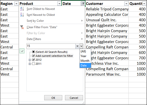
Figure 8.5. With proper use of the additive search property, you can easily create a report of specific dates.

Because searches are additive, proper application of the Add Current Selection to Filter in the search results allows you to include or exclude the results from the filter. For more information, see the section “Using the Search Function to Filter for or Exclude Items.”

You need to create a report with all the records from the first of every month available in 2011 and the 15^th of every month in 2012. Using the additive search property, you can quickly filter to those specific records. To do so, follow these steps:

1. Open the drop-down of the Date column to filter.

2. Select Date from the Search drop-down.

3. Type in the two-digit date, 01.

4. Because the results are open to show everything, scroll to the top of the list and click the + by the years to minimize the list.

5. Deselect 2012 and click OK. The results now show all the first of the month records from 2011.

6. Open the drop-down of the Date column to filter again.

7. Select Date from the Search drop-down.

8. Type in the two-digit date, 15.

9. Scroll to the top and deselect Select All Search Results.

10. Select 2012 to select all 2012 results.

11. Select Add Current Selection to Filter, as shown in Figure 8.5.

12. Click OK.

Using Text, Number, and Date Special Filters

With careful planning or additional columns, you can filter for all types of reports such as top 10, quarterly reports, and ranges of values. But not all filtering is easy or quick. The filter listing has options to make it easier. Special filters are available in the filter drop-down depending on which data type (text, numbers, or dates) appears most often in a column. All the special filters, except for ones that take action immediately, open the Custom AutoFilter dialog box, allowing two conditions to be combined using AND or OR.

If the column contains mostly text, Text Filters is available from the filter listing. Choosing Text Filters opens a list with the following options: Equals, Does Not Equal, Begins With, Ends With, Contains, and Does Not Contain. Selecting one of these options opens a Custom AutoFilter dialog box, in which you can enter text to filter by.

If the column contains mostly numbers, Number Filters is available with the following options: Equals, Does Not Equal, Greater Than, Greater Than Or Equal To, Less Than, Less Than or Equal To, Between Top 10, Above Average, and Below Average. Selecting Top 10, Above Average, or Below Average automatically updates the filter to reflect the selection.

If Top 10 is selected, you can specify the top or bottom items or percent to view. For example, you could choose to view the bottom 15% or the top seven items.

For columns with dates, the special filter, Date Filters, offers a wide selection of options, including additional options under All Dates in the Period. The options dealing with quarters refer to the traditional quarter of a year, January through March being the first quarter, April through June being the second quarter, and so on. When using the Custom AutoFilter option, the dialog box for dates includes calendars to aid in data entry.

To create the bottom 25% report for the previous quarter shown in Figure 8.6, follow these steps:

1. Open the drop-down of the Date column.

2. Select Date Filters, All Dates in the Period, Quarter 2. The data automatically filters to the 2nd quarter, April–June.

3. Open the drop-down of the numeric column, Quantity, to filter.

4. Select Number Filters, Top 10. The Top 10 AutoFilter appears.

5. Select Bottom from the leftmost drop-down.

6. Enter 25 in the middle field.

7. Select Percent from the rightmost drop-down.

8. Click OK; the table filters show the bottom 25%.

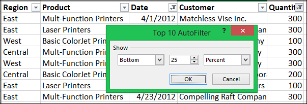
Figure 8.6. The special filters make it easier to create quarterly reports reflecting records that fall within specific parameters.

Filtering by Color or Icon

Data can be filtered by font color, color (set by cell fill or conditional formatting), or icon by going to the Filter by Color option in the filter listing. There, colors and/or icons used in the column are listed, as shown in Figure 8.7.

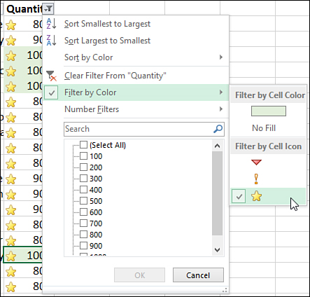
Figure 8.7. You can filter by the colors and icons in the table.

The data table in Figure 8.7 uses conditional formatting icons to denote which record quantities are below average (arrow), average (exclamation mark), or above average (star). Also, quantities greater than or equal to 1,000 have a green cell fill. To filter to show only the above average items, open the drop-down filter for the Quantity column. Select Filter by Color and then from the icons listed, select the star. The list automatically updates to show only the star records.

Filtering by Selection

Even without the filter turned on, you can right-click any cell in a column, go to Filter, and choose to filter by the cell’s value, color, font color, or icon. Doing so turns on the AutoFilter and configures the filter for the selected cell’s property.

This filtering is additive. If you filter a cell by one value and then go to a cell in another column and filter by its value, the result will be those rows that satisfy both filter criteria. You cannot filter by a property more than once within the same column, but you can filter a column by multiple properties—for example, filter by icon and then value.

To use filter selection to filter records meeting a specific value and icon, such as the below average East records in Figure 8.8, follow these steps:

1. Right-click a cell in the Region column containing the value (East) to filter by.

2. Go to Filter, Filter by Selected Cell’s Value. The AutoFilter drop-downs appear in the column header and the table updates to show only East records.

3. Right-click a cell in the Quantity column containing the icon (a down arrow) to filter by.

4. Go to Filter, Filter by Selected Cell’s Icon. The table now shows all below average records from the East region.

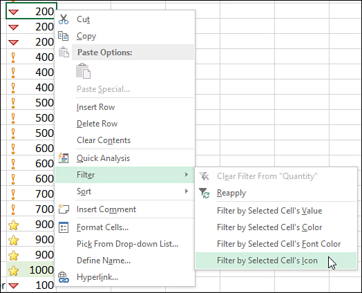
Figure 8.8. Right-clicking on a specific cell allows you to quickly filter by that cell’s value, cell color, font color, or icon.

Allowing Filtering on a Protected Sheet

Normally, if you set up filters on a sheet, protect the sheet, and then send it out to other users, the recipients won’t be able to filter the data. If you want others to be able to filter your protected sheet, follow these steps:

1. Select a single cell in the data set to apply filtering to.

2. Go to Home, Sort & Filter, Filter. The filter will be turned on for the data set.

3. Go to Review, Changes, Protect Sheet.

4. In the listing for Allow All Users of This Worksheet To, scroll down and select Use AutoFilter.

5. If applying a password to the sheet, enter it in the Password to Unprotect Sheet field. Otherwise, skip to step 6.

6. Click OK.

7. If you entered a password in step 5, Excel prompts you to reenter the password. Do so and click OK.

Users won’t be able to modify the data you’ve protected, but they’ll be able to use Excel’s various AutoFilter tools to filter the data as needed.

Using the Advanced Filter Option

Advanced Filter, found under Data, Sort & Filter, Advanced, may be a bit of a misnomer. Despite the visual simplicity of the Advanced Filter dialog box, shown in Figure 8.9, it can perform a variety of functions. Depending on the options selected and the setup on the sheet, the Advanced Filter can do the following:

• Filter records in place

• Filter records to a new location on the same or different sheet

• Reorganize columns

• Use formulas as criteria

• Filter for unique records

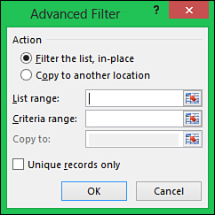
Figure 8.9. With proper use of the Advanced Filter dialog box, you can do more than filter your data.

Under Action, you can choose either Filter the List, In-Place or Copy to Another Location to tell the function where to put the resulting data set. If copying the results to a new location, specify the location in the Copy To field. When specifying this range, consider the following:

• If the results include all columns of the data set in the original order, only the location of the first header needs to be specified.

• If the results consist of any change to the headers, whether it’s a new order or fewer headers, copy the headers to use in the desired order to a new location. The Copy To range must include the entire new range of headers.

• If results need to be on another sheet, the Advanced Filter must be called from the sheet where the results will be placed.

List Range is the data set, including required headers. Most Advanced Filter functions require each column to have a header.

Criteria Range is where rules are configured for the filter. See “Filtering by Criteria Range” for details.

Select Unique Records Only if duplicates should not be included in the results. See “Creating a List of Unique Items” for an example of how the option is useful for removing duplicates from a single column.

Filtering by Criteria Range

Criteria are the rules you want to execute the filter by. It’s an optional field. Criteria can consist of exact values, values with operators, wildcards, or formulas. You should keep the following things in mind when setting up the criteria range:

• Except for when the criterion is a formula, the first row must consist of the column header used by the filter.

• Starting in the second row, enter the criterion to filter for in the column.

• Criteria entered on the same row are read as joined by AND. In the top table of Figure 8.10, the criteria in the first row are read West AND Laser Printers.

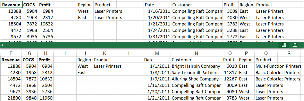
Figure 8.10. The top table shows the criteria properly configured to return all Laser Printers for West and East regions. The configuration of the bottom table’s criteria will return Laser Printers for West, but all products for East.

• Criteria entered on different rows are read as joined by OR. In the top table of Figure 8.10, the criteria are read West AND Laser Printers OR East AND Laser Printers.

• If a cell in the criteria range is blank and has a column header, this is read as returning all records that match the column header. In the bottom table in Figure 8.10, the data returned will be West and Laser Printers or all data in East.

• Operators (<, >, <=, >=, <>) can be combined with numeric values for a more general filter.

• Wildcards can be used with text values. An asterisk (*) replaces any number of characters. A question mark (?) replaces a single character. The tilde (~) allows the use of wildcard characters in case the text being filtered uses such a character as part of its value.

• If the criterion is a formula, do not use a column header as it is applied to the entire data set. The formula should be one that returns TRUE or FALSE.

You can combine the header criteria with formulas to create your report. For example, you need to create a report of region west customers from whom you generated more than $4,000 in profit by selling Laser Printers. Your data spans a couple of years, so you want to narrow those results down to February and March of the current year. You also want to return any non-west region profits from January of the current year. Finally, you want the report generated on a new sheet.

First, you’ll need to set up the header criteria:

1. Starting in G1, enter the headers you want to filter by: Region, Product, Profit. The text must match exactly, so if in doubt of the spelling, copy and paste the titles.

2. Under each column header, in row 2, enter the filter values: West, Laser Printers, >4000.

Next, create the criteria formulas. The one to be applied with the West column criteria needs to be entered in the same row and in an adjacent column (J). The second formula should be entered directly beneath the first.

3. In J2, place the following formula:

=AND(YEAR(C2)=YEAR(TODAY()),OR(MONTH(C2)=2,MONTH(C2)=3))

4. In J3, place the following formula:

=AND(A2<>"West",YEAR(C2)=YEAR(TODAY()),MONTH(C2)=1)

Notice that both formulas were written referring to the first row of data and used relative referencing. Finally, set up the Report sheet and configure the Advanced Filter dialog box, as shown in Figure 8.11.

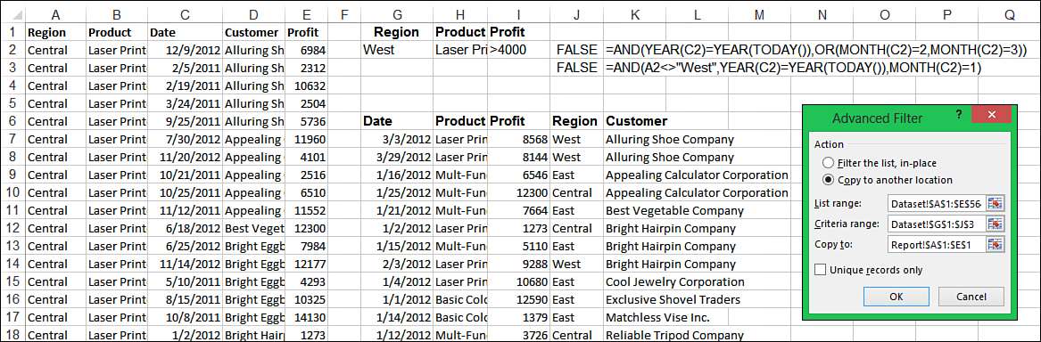
Figure 8.11. The Advanced Filter can use a combination of criteria to filter a data set. Note: Results in G6:K18 are a representation of the actual results on the Report sheet.

5. On the Report sheet, enter the column headings to include in the report: Date, Product, Profit, Region, Customer.

6. Because the results are on a sheet other than the data sheet, we need to start the Filter dialog box from the report sheet. Select a blank cell on the report sheet that is not directly beneath the headings.

7. Go to Data, Sort & Filter, Advanced.

8. Select Copy to Another Location.

9. Place the cursor in the List Range field and select the data set sheet. Select the entire data table.

10. Place the cursor in the Criteria Range field. You will be brought back to the report sheet, so return to the data set sheet.

11. Select the criteria range, including the headers. Do not include any blank rows.

12. Place the cursor in the Copy To field. You are brought back to the report sheet.

13. Select the column headers on the report sheet.

14. Click OK. The report sheet updates with the results.

Creating a List of Unique Items

When the Unique Records Only option is selected, the Advanced Filter can be used to remove duplicates. Unlike the Remove Duplicates command on the Data tab, the original data set remains intact if you choose to copy the results to a new location. But also unlike the Remove Duplicates command, you cannot specify multiple columns to filter by. The Advanced Filter automatically looks at all columns in the List Range field.

If Filter the List, In-Place is selected, the duplicate rows will be hidden. Go to Data, Sort & Filter, Clear to clear the filter and unhide the rows.

The table in Figure 8.12 shows two years of sales. You need to generate a list of companies products were sold to in that time. To quickly filter out duplicates in the Customer column and copy the results to a new location, follow these steps:

1. Select a cell outside the data table.

2. Go to Data, Sort & Filter, Advanced Filter.

3. Place the cursor in the List Range field.

4. Select the column to create the unique listing from, column D. As long as you don’t have another table beneath this one, you can select the entire column by clicking on the header.

5. Select Copy to Another Location.

6. Place your cursor in the Copy To field.

7. Select a cell on the sheet where you want the first cell of the filtered range copied to, for example, J1.

8. Select Unique Records Only.

9. Click OK. A list of all unique customers is generated, as shown in Figure 8.12.

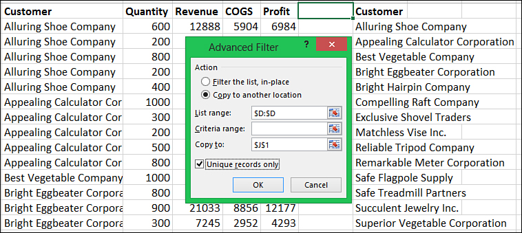
Figure 8.12. Use the Advanced Filter to create a unique list of items from your data set.

Removing Duplicates from a Data Set

You’ve received a report where a user duplicated data by importing twice. You could try sorting the data and creating a formula in another column that compares rows, but with over 700,000 rows, it could take a while for the formula to calculate and you aren’t even sure if the process is foolproof. Instead, use the Remove Duplicates option to ensure the process. Remove Duplicates can be found under Data, Data Tools, Remove Duplicates, or if the data set is a Table, under Table Tools, Design, Tools, Remove Duplicates.

To remove duplicates based on the Region, Product, Date, and Customer, follow these steps:

1. Select a cell in the data set.

2. Go to Data, Data Tools, Remove Duplicates.

3. Excel highlights the data set. If columns are missing in the selection, go back and make sure there are no blank separating columns.

4. From the Remove Duplicates dialog box, make sure My Data Has Headers is selected if the data set has headers.

5. By default, all the columns are selected. A selected column means the tool will use the columns when looking for duplicates. Duplicates in an unselected column will be ignored. In the Columns list box, select the columns to use in the search for duplicates, as shown in Figure 8.13.

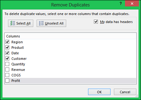
Figure 8.13. Remove Duplicates allows you to specify which columns you want to use to verify duplicate records.

6. Click OK. The data set updates, deleting any duplicate rows. A message box appears informing you of the number of rows deleted and the number remaining in the data set.

Consolidating Data

The Remove Duplicates tool is great for completely removing duplicates, but what if you wanted to remove duplicates based on some fields and, at the same time, combine the data of other fields? For example, you have a sheet with 2011 data and a sheet with 2012 data. You need to create a quantity sold report combining the data based on the company name but separating the different years. You could create a pivot table or use the Consolidate tool. The Consolidate tool, found under Data, Data Tools, helps you create a report of unique records with combined data. It even combines data from different sheets and workbooks. You can do this in one of three ways:

• By Position—Sum¹ data found on different sheets or in different workbooks based on their positions in the data sets. For example, if the ranges are A1:A10 and C220:C230, the results will be A1+C220, A2+C221, A3+C222, and so on. Do not select either of the options under Use Labels In.

• By Category—Sum¹ data found on different sheets or in different workbooks based on matching row and column labels, similar to a pivot table report. The references must include the labels in the leftmost column of the ranges. Select either or both of the options under Use Labels In to have the labels appear in the final data.

¹The function applied to the data can be any listed in the drop-down in the Consolidate dialog box. These include Sum, Count, Average, and more.

• By Column—Combine the data to a new sheet, with each data set in its own column. Select the Top Row option under Use Labels In.

The Reference field is where the data sets are entered. Click Add to add the selection to the All References list. If the data set is in a closed workbook, you can reference it only by using a range name. Click the Browse button to find and select the workbook. After the exclamation point (!) at the end of the path, enter the range name assigned to the data set.

If Create Links to Source Data is selected, the consolidated data updates automatically when the source is changed. Also, the consolidated data is grouped, as shown in Figure 8.14. Click the + icon to the left of the data to open the group and see the data used in the summary. Column B of the report shows the name of the workbook in the first instance of its data.

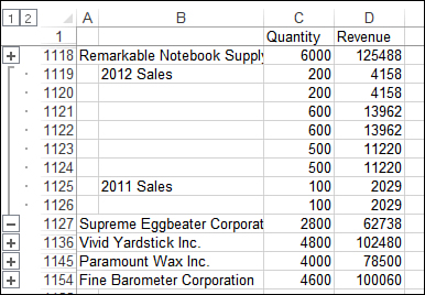
Figure 8.14. When Create Links to Source Data is selected, the final report includes the individual values of the selected references.

A few things to keep in mind when using this tool:

• The range selected must be adjacent columns.

• If your reference field consists of multiple sheets, as you go from sheet to sheet, Excel automatically selects the same range as the previous sheet.

• If you select Left column, data is combined based on the leftmost column of the selection and the selected function is used on all other columns in the range.

• If doing a consolidatation by position or by column, you have to select a specific range, versus clicking the column headers to select the entire column.

• The range on which the function is applied must be numerical.

You have two reports, sales from 2011 and sales from 2012 on separate sheets. To combine the customers and the quantity sold onto a single report, follow these steps:

1. Select the top leftmost cell where the consolidated report should be placed, such as cell A1. If other data is on the sheet, make sure there is enough room for the new data.

2. Go to Data, Data Tools, Consolidate.

3. Select the desired function, SUM, from the Function drop-down.

4. Place the cursor in the Reference field.

5. Go to the sheet with the desired data set.

6. Select the data set, making sure the labels to be combined are in the leftmost column and that the column headers are included in the selection.

7. Click the Add button.

8. Repeat steps 4 to 7 for each additional data set, as shown in Figure 8.15.

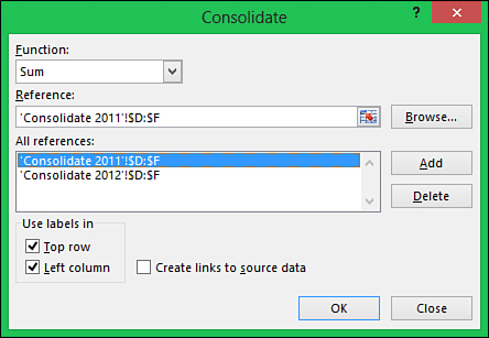
Figure 8.15. Use Consolidate to combine records from multiple sheets into a single report.

9. To include the top and/or left column labels, select the corresponding option. If combining text fields, as we are here, Left Column must be selected.

10. Click OK.