
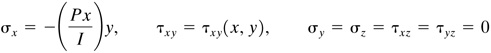
Chapter 3. Two-Dimensional Problems in Elasticity
3.1 Introduction
As has been pointed out in Sec. 1.1, the approaches in widespread use for determining the influence of applied loads on elastic bodies are the mechanics of materials or elementary theory (also known as technical theory) and the theory of elasticity. Both must rely on the conditions of equilibrium and make use of a relationship between stress and strain that is usually considered to be associated with elastic materials. The essential difference between these methods lies in the extent to which the strain is described and in the types of simplifications employed.
The mechanics of materials approach uses an assumed deformation mode or strain distribution in the body as a whole and hence yields the average stress at a section under a given loading. Moreover, it usually treats separately each simple type of complex loading, for example, axial centric, bending, or torsion. Although of practical importance, the formulas of the mechanics of materials are best suited for relatively slender members and are derived on the basis of very restrictive conditions. On the other hand, the method of elasticity does not rely on a prescribed deformation mode and deals with the general equations to be satisfied by a body in equilibrium under any external force system.
The theory of elasticity is preferred when critical design constraints such as minimum weight, minimum cost, or high reliability dictate more exact treatment or when prior experience is limited and intuition does not serve adequately to supply the needed simplifications with any degree of assurance. If properly applied, the theory of elasticity should yield solutions more closely approximating the actual distribution of strain, stress, and displacement.
Thus, elasticity theory provides a check on the limitations of the mechanics of materials solutions. We emphasize, however, that both techniques cited are approximations of nature, each of considerable value and each supplementing the other. The influences of material anisotropy, the extent to which boundary conditions depart from reality, and numerous other factors all contribute to error.
3.2 Fundamental Principles of Analysis
To ascertain the distribution of stress, strain, and displacement within an elastic body subject to a prescribed system of forces requires consideration of a number of conditions relating to certain physical laws, material properties, and geometry. These fundamental principles of analysis, also referred to as the three aspects of solid mechanics problems, are summarized as follows:
1. Conditions of equilibrium. The equations of statics must be satisfied throughout the body.
2. Stress–strain relations. Material properties (constitutive relations, for example, Hooke’s law) must comply with the known behavior of the material involved.
3. Conditions of compatibility. The geometry of deformation and the distribution of strain must be consistent with the preservation of body continuity. (The matter of compatibility is not always broached in mechanics of materials analysis.)
In addition, the stress, strain, and displacement fields must be such as to conform to the conditions of loading imposed at the boundaries. This is known as satisfying the boundary conditions for a particular problem. If the problem is dynamic, the equations of equilibrium become the more general conservation of momentum; conservation of energy may be a further requirement.
The conditions described, and stated mathematically in the previous chapters, are used to derive the equations of elasticity. In the case of a three-dimensional problem in elasticity, it is required that the following 15 quantities be ascertained: six stress components, six strain components, and three displacement components. These components must satisfy 15 governing equations throughout the body in addition to the boundary conditions: three equations of equilibrium, six stress–strain relations, and six strain–displacement relations. Note that the equations of compatibility are derived from the strain–displacement relations, which are already included in the preceding description. Thus, if the 15 expressions are satisfied, the equations of compatibility will also be satisfied. Three-dimensional problems in elasticity are often very complex. It may not always be possible to use the direct method of solution in treating the general equations and given boundary conditions. Only a useful indirect method of solution will be presented in Secs. 6.3 and 6.4.
In many engineering applications, ample justification may be found for simplifying assumptions with respect to the state of strain and stress. Of special importance, because of the resulting decrease in complexity, are those reducing a three-dimensional problem to one involving only two dimensions. In this regard, we shall discuss throughout the text various plane strain and plane stress problems.
This chapter is subdivided into two parts. In Part A, derivations of the governing differential equations and various approaches for solution of two-dimensional problems in Cartesian and polar coordinates are considered. Part B treats stress concentrations in members whose cross sections manifest pronounced changes and cases of load application over small areas.
Part A—Formulation and Methods of Solution
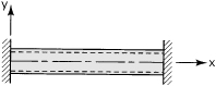
3.3 Plane Strain Problems
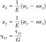
Consider a long prismatic member subject to lateral loading (for example, a cylinder under pressure), held between fixed, smooth, rigid planes (Fig. 3.1). Assume the external force to be functions of the x and y coordinates only. As a consequence, we expect all cross sections to experience identical deformation, including those sections near the ends. The frictionless nature of the end constraint permits x, y deformation, but precludes z displacement; that is, w = 0 at z = ±L/2. Considerations of symmetry dictate that w must also be zero at midspan. Symmetry arguments can again be used to infer that w = 0 at ±L/4, and so on, until every cross section is taken into account. For the case described, the strain depends on x and y only:
(3.1)
![]()
(3.2)
![]()
Figure 3.1. Plane strain in a cylindrical body.

The latter expressions depend on ∂u/∂z and ∂υ/∂z vanishing, since w and its derivatives are zero. A state of plane strain has thus been described wherein each point remains within its transverse plane, following application of the load. We next proceed to develop the equations governing the behavior of bodies under plane strain.
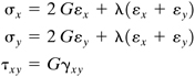
Substitution of εz = γyz =γxz = 0 into Eq. (2.30) provides the following stress–strain relationships:
and
(3.4)
![]()
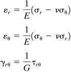
Because σz is not contained in the other governing expressions for plane strain, it is determined independently by applying Eq. (3.4). The strain-stress relations, Eqs. (2.28), for this case become
(3.5)

Inasmuch as these stress components are functions of x and y only, the first two equations of (1.11) yield the following equations of equilibrium of plane strain:
(3.6)

The third equation of (1.11) is satisfied if Fz = 0. In the case of plane strain, therefore, no body force in the axial direction can exist.
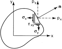
A similar restriction is imposed on the surface forces. That is, plane strain will result in a prismatic body if the surface forces px and py are each functions of x and y and pz = 0. On the lateral surface, n = 0 (Fig. 3.2). The boundary conditions, from the first two equations of (1.41), are thus given by
(3.7)
![]()
Figure 3.2. Surface forces.
Clearly, the last equation of (1.41) is also satisfied.
In the case of a plane strain problem, therefore, eight quantities, σx, σy, τxy, εx, εy, γxy, u, and υ, must be determined so as to satisfy Eqs. (3.1), (3.3), and (3.6) and the boundary conditions (3.7). How eight governing equations, (3.1), (3.3), and (3.6), may be reduced to three is now discussed.
Three expressions for two-dimensional strain at a point [Eq. (3.1)] are functions of only two displacements, u and υ, and therefore a compatibility relationship exists among the strains [Eq. (2.8)]:
(3.8)
![]()
This equation must be satisfied for the strain components to be related to the displacements as in Eqs. (3.1). The condition as expressed by Eq. (3.8) may be transformed into one involving components of stress by substituting the strain-stress relations and employing the equations of equilibrium. Performing the operations indicated, using Eqs. (3.5) and (3.8), we have
(a)
![]()
Next, the first and second equations of (3.6) are differentiated with respect to x and y, respectively, and added to yield
![]()
Finally, substitution of this into Eq. (a) results in
(3.9)
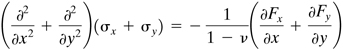
This is the equation of compatibility in terms of stress.
We now have three expressions, Eqs. (3.6) and (3.9), in terms of three unknown quantities: σx, σy, and τxy. This set of equations, together with the boundary conditions (3.7), is used in the solution of plane strain problems. For a given situation, after determining the stress, Eqs. (3.5) and (3.1) yield the strain and displacement, respectively. In Sec. 3.5, Eqs. (3.6) and (3.9) will further be reduced to one equation containing a single variable.
3.4 Plane Stress Problems
In many problems of practical importance, the stress condition is one of plane stress. The basic definition of this state of stress has already been given in Sec. 1.8. In this section we shall present the governing equations for the solution of plane stress problems.
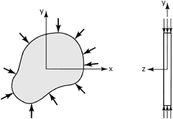
To exemplify the case of plane stress, consider a thin plate, as in Fig. 3.3, wherein the loading is uniformly distributed over the thickness, parallel to the plane of the plate. This geometry contrasts with that of the long prism previously discussed, which is in a state of plane strain. To arrive at tentative conclusions with regard to the stress within the plate, consider the fact that σz, τxz, and τyz are zero on both faces of the plate. Because the plate is thin, the stress distribution may be very closely approximated by assuming that the foregoing is likewise true throughout the plate.
Figure 3.3. Thin plate under plane stress.
We shall, as a condition of the problem, take the body force Fz = 0 and Fx and Fy each to be functions of x and y only. As a consequence of the preceding, the stress is specified by
(a)
![]()
The nonzero stress components remain constant over the thickness of the plate and are functions of x and y only. This situation describes a state of plane stress. Equations (1.11) and (1.41), together with this combination of stress, again reduce to the forms found in Sec. 3.3. Thus, Eqs. (3.6) and (3.7) describe the equations of equilibrium and the boundary conditions in this case, as in the case of plane strain.
Substitution of Eq. (a) into Eq. (2.28) yields the following stress–strain relations for plane stress:
(3.10)
and
(3.11a)
![]()
Solving for σx + σy from the sum of the first two of Eqs. (3.10) and inserting the result into Eq. (3.11a), we obtain
(3.11b)
![]()
Equations (3.11) define the out-of-plane principal strain in terms of the in-plane stresses (σx, σy) or strains (εx, εy).
Because εz is not contained in the other governing expressions for plane stress, it can be obtained independently from Eqs. (3.11); then εz = ∂w/∂z may be applied to yield w. That is, only u and υ are considered as independent variables in the governing equations. In the case of plane stress, therefore, the basic strain–displacement relations are again given by Eqs. (3.1). Exclusion from Eq. (2.3) of εz = ∂w/∂z makes the plane stress equations approximate, as is demonstrated in the section that follows.
The governing equations of plane stress will now be reduced, as in the case of plane strain, to three equations involving stress components only. Since Eqs. (3.1) apply to plane strain and plane stress, the compatibility condition represented by Eq. (3.8) applies in both cases. The latter expression may be written as follows, substituting strains from Eqs. (3.10) and employing Eqs. (3.6):
(3.12)
![]()
This equation of compatibility, together with the equations of equilibrium, represents a useful form of the governing equations for problems of plane stress.
To summarize the two-dimensional situations discussed, the equations of equilibrium [Eqs. (3.6)], together with those of compatibility [Eq. (3.9) for plane strain and Eq. (3.12) for plane stress] and the boundary conditions [Eqs. (3.7)], provide a system of equations sufficient for determination of the complete stress distribution. It can be shown that a solution satisfying all these equations is, for a given problem, unique [Ref. 3.1]. That is, it is the only solution to the problem.
In the absence of body forces or in the case of constant body forces, the compatibility equations for plane strain and plane stress are the same. In these cases, the equations governing the distribution of stress do not contain the elastic constants. Given identical geometry and loading, a bar of steel and one of Lucite should thus display identical stress distributions. This characteristic is important in that any convenient isotropic material may be used to substitute for the actual material, as, for example, in photoelastic studies.
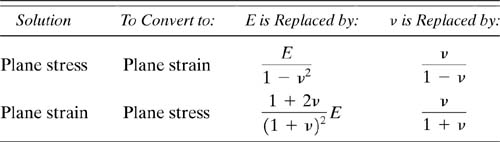
It is of interest to note that by comparing Eqs. (3.5) with Eqs. (3.10) we can form Table 3.1, which facilitates the conversion of a plane stress solution into a plane strain solution, and vice versa. For instance, conditions of plane stress and plane strain prevail in a narrow beam and a very wide beam, respectively. Hence, in a result pertaining to a thin beam, EI would become EI/(1 – ν2) for the case of a wide beam. The stiffness in the latter case is, for ν = 0.3, about 10% greater owing to the prevention of sidewise displacement (Secs. 5.2 and 13.3).
3.5 Airy’s Stress Function
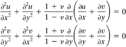
The preceding sections have demonstrated that the solution of two-dimensional problems in elasticity requires integration of the differential equations of equilibrium [Eqs. (3.6)], together with the compatibility equation [Eq. (3.9) or (3.12)] and the boundary conditions [Eqs. (3.7)]. In the event that the body forces Fx and Fy are negligible, these equations reduce to
(a)
![]()
(b)
together with the boundary conditions (3.7). The equations of equilibrium are identically satisfied by the stress function, Φ(x, y), introduced by G. B. Airy, related to the stresses as follows:
(3.13)
![]()
Substitution of (3.13) into the compatibility equation, Eq. (b), yields
(3.14)
![]()
What has been accomplished is the formulation of a two-dimensional problem in which body forces are absent, in such a way as to require the solution of a single biharmonic equation, which must of course satisfy the boundary conditions.
It should be noted that in the case of plane stress we have σZ = τxz = τyz = 0 and σx, σy, and τxy independent of z. As a consequence, γxz = γyz = 0, and εx, εy, εz, and γxy are independent of z. In accordance with the foregoing, from Eq. (2.9), it is seen that in addition to Eq. (3.14), the following compatibility equations also hold:
(c)
![]()
Clearly, these additional conditions will not be satisfied in a case of plane stress by a solution of Eq. (3.14) alone. Therefore, such a solution of a plane stress problem has an approximate character. However, it can be shown that for thin plates the error introduced is negligibly small.
It is also important to note that, if the ends of the cylinder shown in Fig. 3.1 are free to expand, we may assume the longitudinal strain εz to be a constant. Such a state may be called that of generalized plane strain. Therefore, we now have
(3.15)
and
(3.16)
![]()
Introducing Eqs. (3.15) into Eq. (3.8) and simplifying, we again obtain Eq. (3.14) as the governing differential equation. Having determined σx and σy, the constant value of εz, can be found from the condition that the resultant force in the z direction acting on the ends of the cylinder is zero. That is,
(d)
![]()
where σz is given by Eq. (3.16).
3.6 Solution of Elasticity Problems
Unfortunately, solving directly the equations of elasticity derived may be a formidable task, and it is often advisable to attempt a solution by the inverse or semi-inverse method. The inverse method requires examination of the assumed solutions with a view toward finding one that will satisfy the governing equations and boundary conditions. The semi-inverse method requires the assumption of a partial solution formed by expressing stress, strain, displacement, or stress function in terms of known or undetermined coefficients. The governing equations are thus rendered more manageable.
It is important to note that the preceding assumptions, based on the mechanics of a particular problem, are subject to later verification. This is in contrast with the mechanics of materials approach, in which analytical verification does not occur. The applications of inverse, semi-inverse, and direct methods are found in examples to follow and in Chapters 5, 6, and 8.
A number of problems may be solved by using a linear combination of polynomials in x and y and undetermined coefficients of the stress function Φ. Clearly, an assumed polynomial form must satisfy the biharmonic equation and must be of second degree or higher in order to yield a nonzero stress solution of Eq. (3.13), as described in the following paragraphs. In general, finding the desirable polynomial form is laborious and requires a systematic approach [Refs. 3.2 and 3.3]. The Fourier series, indispensible in the analytical treatment of many problems in the field of applied mechanics, is also often employed (Secs. 10.10 and 13.6).
Another way to overcome the difficulty involved in the solution of Eq. (3.14) is to use the method of finite differences. Here the governing equation is replaced by series of finite difference equations (Sec. 7.3), which relate the stress function at stations that are removed from one another by finite distances. These equations, although not exact, frequently lead to solutions that are close to the exact solution. The results obtained are, however, applicable only to specific numerical problems.
Polynomial Solutions
An elementary approach to obtaining solutions of the biharmonic equation uses polynomial functions of various degree with their coefficients adjusted so that ∇4Φ = 0 is satisfied. A brief discussion of this procedure follows.
A polynomial of the second degree,
(3.17)
![]()
satisfies Eq. (3.14). The associated stresses are
![]()
All three stress components are constant throughout the body. For a rectangular plate (Fig. 3.4a), it is apparent that the foregoing may be adapted to represent simple tension (c2 ≠ 0), double tension (c2 ≠ 0, a2 ≠ 0), or pure shear (b2 ≠ 0).
Figure 3.4. Stress fields of (a) Eq. (3.17) and (b) Eq. (3.18).

A polynomial of the third degree
(3.18)
![]()
fulfills Eq. (3.14). It leads to stresses
![]()
For a3 = b3 = c3 = 0, these expressions reduce to
![]()
representing the case of pure bending of the rectangular plate (Fig. 3.4b).
A polynomial of the fourth degree,
(3.19)
![]()
satisfies Eq. (3.14) if e4 = −(2c4 + a4). The corresponding stresses are

A polynomial of the fifth degree
(3.20)
![]()
fulfills Eq. (3.14) provided that
(3a5 + 2c5 + e5)x + (b5 + 2d5 + 3f5)y = 0
It follows that
![]()
The components of stress are then
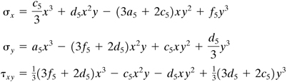
Problems of practical importance may be solved by combining functions (3.17) through (3.20), as required. With experience, the analyst begins to understand the types of stress distributions arising from a variety of polynomials.
Example 3.1
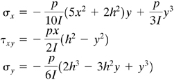
A narrow cantilever of rectangular cross section is loaded by a concentrated force at its free end of such magnitude that the beam weight may be neglected (Fig. 3.5a). Determine the stress distribution in the beam.
Figure 3.5. Example 3.1. End-loaded cantilever beam.
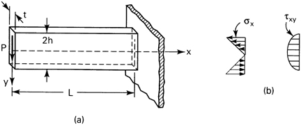
Solution The situation described may be regarded as a case of plane stress provided that the beam thickness t is small relative to the beam depth 2h.
The following boundary conditions are consistent with the coordinate system in Fig. 3.5a:
(a)
![]()
These conditions simply express the fact that the top and bottom edges of the beam are not loaded. In addition to Eq. (a) it is necessary, on the basis of zero external loading in the x direction at x = 0, that σx = 0 along the vertical surface at x = 0. Finally, the applied load P must be equal to the resultant of the shearing forces distributed across the free end:
![]()
The negative sign agrees with the convention for stress discussed in Sec. 1.4.
For purposes of illustration, three approaches will be employed to determine the distribution of stress within the beam.
Method 1. Inasmuch as the bending moment varies linearly with x and σx at any section depends on y, it is reasonable to assume a general expression of the form
(c)
![]()
in which C1 represents a constant. Integrating twice with respect to y,
(d)
![]()
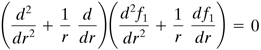
where f1(x) and f2(x) are functions of x to be determined. Introducing the Φ thus obtained into Eq. (3.14), we have
![]()
Since the second term is independent of y, a solution exists for all x and y provided that d4f1/dx4 = 0 and d4f2/dx4 = 0, which, upon integrating, leads to
f1(x) = c2x3 + c3x2 + c4x + c5
f2(x) = c6x3 + c7x2 + c8x + c9
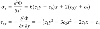
where c2, c3,…, are constants of integration. Substitution of f1(x) and f2(x) into Eq. (d) gives
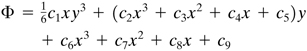
Expressions for σy and τxy follow from Eq. (3.13):
(e)
At this point, we are prepared to apply the boundary conditions. Substituting Eqs. (a) into (e), we obtain c2 = c3 = c6 = c7 = 0 and ![]() . The final condition, Eq. (b), may now be written as
. The final condition, Eq. (b), may now be written as
![]()
from which
![]()
where I = ![]() th3 is the moment of inertia of the cross section about the neutral axis. From Eqs. (c) and (e), together with the values of the constants, the stresses are found to be
th3 is the moment of inertia of the cross section about the neutral axis. From Eqs. (c) and (e), together with the values of the constants, the stresses are found to be
(3.21)
![]()
The distribution of these stresses at sections away from the ends is shown in Fig. 3.5b.
Method 2. Beginning with bending moments Mz = Px, we may assume a stress field similar to that for the case of pure bending:
(f)
Equation of compatibility (3.12) is satisfied by these stresses. On the basis of Eqs. (f), the equations of equilibrium lead to
(g)
![]()
From the second expression, τxy can depend only on y. The first equation of (g) together with Eqs. (f) yields
![]()
from which
![]()
Here c is determined on the basis of (τxy)y + ±h = 0: c = −Ph2/2I. The resulting expression for τxy satisfies Eq. (b) and is identical with the result previously obtained.
Method 3. The problem may be treated by superimposing the polynomials Φ2 and Φ4,
a2 = c2 = a4 = b4 = c4 = e4 = 0
Thus,
![]()
The corresponding stress components are
![]()
It is seen that the foregoing satisfies the second condition of Eqs. (a). The first of Eqs. (a) leads to d4 = −2b2/h2. We then obtain

which when substituted into condition (b) results in b2 = −3P/4ht = Ph2/2I. As before, τxy is as given in Eqs. (3.21).
Observe that the stress distribution obtained is the same as that found by employing the elementary theory. If the boundary forces result in a stress distribution as indicated in Fig. 3.5b, the solution is exact. Otherwise, the solution is not exact. In any case, recall, however, that Saint-Venant’s principle permits us to regard the result as quite accurate for sections away from the ends.
Section 5.4 illustrates the determination of the displacement field after derivation of the curvature-moment relation.
3.7 Thermal Stresses
Consider the consequences of increasing or decreasing the uniform temperature of an entirely unconstrained elastic body. The resultant expansion or contraction occurs in such a way as to cause a cubic element of the solid to remain cubic, while experiencing changes of length on each of its sides. Normal strains occur in each direction unaccompanied by normal stresses. In addition, there are neither shear strains nor shear stresses. If the body is heated in such a way as to produce a nonuniform temperature field, or if the thermal expansions are prohibited from taking place freely because of restrictions placed on the boundary even if the temperature is uniform, or if the material exhibits anisotropy in a uniform temperature field, thermal stresses will occur. The effects of such stresses can be severe, especially since the most adverse thermal environments are often associated with design requirements involving unusually stringent constraints as to weight and volume. This is especially true in aerospace applications, but is of considerable importance, too, in many everyday machine design applications.
Solution of thermal stress problems requires reformulation of the stress–strain relationships accomplished by superposition of the strain attributable to stress and that due to temperature. For a change in temperature T(x, y), the change of length, δL, of a small linear element of length L in an unconstrained body is δL = αLT. Here α, usually a positive number, is termed the coefficient of linear thermal expansion. The thermal strain εt associated with the free expansion at a point is then
(3.22)
![]()
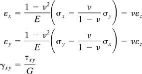
The total x and y strains, εx and εy, are obtained by adding to the thermal strains of the type described, the strains due to stress resulting from external forces:
(3.23a)
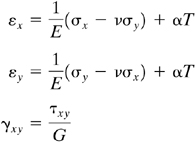
In terms of strain components, these expressions become
(3.23b)
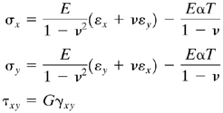
Because free thermal expansion results in no angular distortion in an isotropic material, the shearing strain is unaffected, as indicated. Equations (3.23) represent modified strain-stress relations for plane stress. Similar expressions may be written for the case of plane strain. The differential equations of equilibrium (3.6) are based on purely mechanical considerations and are unchanged for thermoelasticity. The same is true of the strain–displacement relations (2.3) and the compatibility equation (3.8), which are geometrical in character. Thus, for given boundary conditions (expressed either as surface forces or displacements) and temperature distribution, thermoelasticity and ordinary elasticity differ only to the extent of the strain-stress relationship.
By substituting the strains given by Eq. (3.23a) into the equation of compatibility (3.8), employing Eq. (3.6) as well, and neglecting body forces, a compatibility equation is derived in terms of stress:
![]()
Introducing Eq. (3.13), we now have
(3.25)
![]()
This expression is valid for plane strain or plane stress provided that the body forces are negligible.
It has been implicit in treating the matter of thermoelasticity as a superposition problem that the distribution of stress or strain plays a negligible role in influencing the temperature field [Refs. 3.4 and 3.5]. This lack of coupling enables the temperature field to be determined independently of any consideration of stress or strain. If the effect of the temperature distribution on material properties cannot be disregarded, the equations become coupled and analytical solutions are significantly more complex, occupying an area of considerable interest and importance. Numerical solutions can, however, be obtained in a relatively simple manner through the use of finite difference methods.
Example 3.2
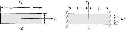
A rectangular beam of small thickness t, depth 2h, and length 2L is subjected to an arbitrary variation of temperature throughout its depth, T = T(y). Determine the distribution of stress and strain for the case in which (a) the beam is entirely free of surface forces (Fig. 3.6a), and (b) the beam is held by rigid walls that prevent the x-directed displacement only (Fig. 3.6b).
Figure 3.6. Example 3.2. Rectangular beam in plane thermal stress: (a) unsupported; (b) placed between two rigid walls.
Solution The beam geometry indicates a problem of plane stress. We begin with the assumptions
(a)
![]()
Direct substitution of Eqs. (a) into Eqs. (3.6) indicates that the equations of equilibrium are satisfied. Equations (a) reduce the compatibility equation (3.24) to the form
(b)
![]()
from which
(c)
![]()
where c1 and c2 are constants of integration. The requirement that faces y = ±h be free of surface forces is obviously fulfilled by Eq. (b).
a. The boundary conditions at the end faces are satisfied by determining the constants that assume zero resultant force and moment at x = ±L:
(d)
![]()
Substituting Eq. (c) into Eqs. (d), it is found that ![]() and
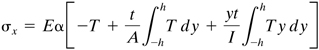
and ![]() . The normal stress, upon substituting the values of the constants obtained, together with the moment of inertia I = 2h3t/3 and area A = 2ht, into Eq. (c) is thus
. The normal stress, upon substituting the values of the constants obtained, together with the moment of inertia I = 2h3t/3 and area A = 2ht, into Eq. (c) is thus
(3.26)
The corresponding strains are
(e)
![]()
The displacements can readily be determined from Eqs. (3.1).
From Eq. (3.26), observe that the temperature distribution for T = constant results in zero stress, as expected. Of course, the strains (e) and the displacements will, in this case, not be zero. It is also noted that, when the temperature is symmetrical about the midsurface (y = 0), that is, T(y) = T(–y), the final integral in Eq. (3.26) vanishes. For an antisymmetrical temperature distribution about the midsurface,T(y) = −T(−y), and the first integral in Eq. (3.26) is zero.
b. For the situation described, εx = 0 for all y. With σy = Txy = 0 and Eq. (c), Eqs. (3.23a) lead to c1 = c2 = 0, regardless of how T varies with y. Thus,
(3.27)
![]()
and
(f)
![]()
Note that the axial stress obtained here can be large even for modest temperature changes, as can be verified by substituting properties of a given material.
3.8 Basic Relations in Polar Coordinates
Geometrical considerations related either to the loading or to the boundary of a loaded system often make it preferable to employ polar coordinates, rather than the Cartesian system used exclusively thus far. In general, polar coordinates are used advantageously where a degree of axial symmetry exists. Examples include a cylinder, a disk, a wedge, a curved beam, and a large thin plate containing a circular hole.
The polar coordinate system (r, θ) and the Cartesian system (x, y) are related by the following expressions (Fig. 3.7a):
(a)
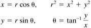
Figure 3.7. (a) Polar coordinates; (b) stress element in polar coordinates.

These equations yield
(b)

Any derivatives with respect to x and y in the Cartesian system may be transformed into derivatives with respect to r and θ by applying the chain rule:
(c)

Relations governing properties at a point not containing any derivatives are not affected by the curvilinear nature of the coordinates, as is observed next.
Equations of Equilibrium
Consider the state of stress on an infinitesimal element abcd of unit thickness described by polar coordinates (Fig. 3.7b). The r and θ-directed body forces are denoted by Fr and Fθ. Equilibrium of radial forces requires that

Inasmuch as dθ is small, sin(dθ/2) may be replaced by dθ/2 and cos(dθ/2) by 1. Additional simplication is achieved by dropping terms containing higher-order infinitesimals. A similar analysis may be performed for the tangential direction. When both equilibrium equations are divided by r dr dθ, the results are
(3.28)

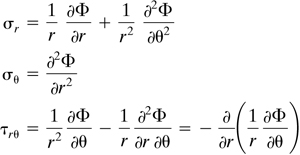
In the absence of body forces, Eqs. (3.28) are satisfied by a stress function Φ(r, θ) for which the stress components in the radial and tangential directions are given by
(3.29)
Strain–Displacement Relations
Consider now the deformation of the infinitesimal element abcd, denoting the r and θ displacements by u and v, respectively. The general deformation experienced by an element may be regarded as composed of (1) a change in length of the sides, as in Figs. 3.8a and b, and (2) rotation of the sides, as in Figs. 3.8c and d.
Figure 3.8. Deformation and displacement of an element in polar coordinates.
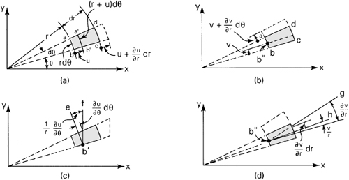
In the analysis that follows, the small angle approximation sin θ ≈ θ is employed, and arcs ab and cd are regarded as straight lines. Referring to Fig. 3.8a, it is observed that a u displacement of side ab results in both radial and tangential strain. The radial strain εr, the deformation per unit length of side ad, is associated only with the u displacement:
(3.30a)
![]()
The tangential strain owing to u, the deformation per unit length of ab, is
(d)
![]()
Clearly, a υ displacement of element abcd (Fig. 3.8b) also produces a tangential strain,
(e)
![]()
since the increase in length of ab is (∂υ/∂θ)dθ. The resultant tangential strain, combining Eqs. (d) and (e), is
(3.30b)
![]()
Figure 3.8c shows the angle of rotation eb′ f of side a′b′ due to a u displacement. The associated strain is
(f)
![]()
The rotation of side bc associated with a υ displacement alone is shown in Fig. 3.8d. Since an initial rotation of b″ through an angle υ/r has occurred, the relative rotation gb″h of side bc is
(g)
![]()
The sum of Eqs. (f) and (g) provides the total shearing strain
![]()
The strain–displacement relationships in polar coordinates are thus given by Eqs. (3.30).
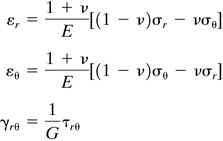
Hooke’s Law
To write Hooke’s law in polar coordinates, we need only replace subscripts x by r and y by θ in the appropriate Cartesian equations. In the case of plane stress, from Eqs. (3.10) we have
(3.31)
For plane strain, Eqs. (3.5) lead to
(3.32)
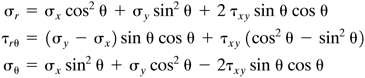
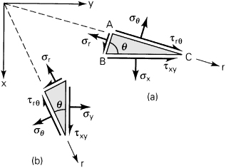
Transformation Equations
Replacement of the subscripts x′ by r and y′ by θ in Eqs. (1.13) results in
(3.33)
We can also express σx, τxy and σy in terms of σr, τrθ, and σθ (Problem 3.26) by replacing θ with −θ in Eqs. (1.13). Thus,
(3.34)
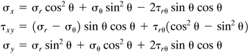
Similar transformation equations may also be written for the strains εr, γrθ and εθ.
Compatibility Equation
It can be shown that Eqs. (3.30) result in the following form of the equation of compatibility:
(3.35)
![]()
To arrive at a compatibility equation expressed in terms of the stress function Φ, it is necessary to evaluate the partial derivatives ∂2Φ/∂x2 and ∂2Φ/∂y2 in terms of r and θ by means of the chain rule together with Eqs. (a). These derivatives lead to the Laplacian operator:
(3.36)
![]()
The equation of compatibility in alternative form is thus
(3.37)
![]()
For the axisymmetrical, zero body force case, the compatibility equation is, from Eq. (3.9) [referring to (3.36)],
(3.38)
![]()
The remaining relationships appropriate to two-dimensional elasticity are found in a manner similar to that outlined in the foregoing discussion.
Example 3.3
A large thin plate is subjected to uniform tensile stress σo at its ends, as shown in Fig. 3.9. Determine the field of stress existing within the plate.
Figure 3.9. Example 3.3. A plate in uniaxial tension.
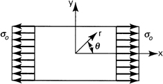
Solution For purposes of this analysis, it will prove convenient to locate the origin of coordinate axes at the center of the plate as shown. The state of stress in the plate is expressed by
![]()
The stress function, Φ = σoy2/2, satisfies the biharmonic equation, Eq. (3.14). The geometry suggests polar form. The stress function Φ may be transformed by substituting y = r sin θ, with the following result:
![]()
The stresses in the plate now follow from Eqs. (h) and (3.29):
(3.39)

Clearly, substitution of σy = τxy = 0 could have led directly to the foregoing result, using the transformation expressions of stress, Eqs. (3.33).
Part B—Stress Concentrations
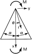
3.9 Stresses Due to Concentrated Loads
Let us now consider a concentrated force P or F acting at the vertex of a very large or semi-infinite wedge (Fig. 3.10). The load distribution along the thickness (z direction) is uniform. The thickness of the wedge is taken as unity, so P or F is the load per unit thickness. In such situations, it is convenient to use polar coordinates and the semi-inverse method.
Figure 3.10. Wedge of unit thickness subjected to a concentrated load per unit thickness: (a) knife edge or pivot; (b) wedge cantilever.

In actuality, the concentrated load is assumed to be a theoretical line load and will be spread over an area of small finite width. Plastic deformation may occur locally. Thus, the solutions that follow are not valid in the immediate vicinity of the application of load.
Compression of a Wedge (Fig. 3.10a).
Assume the stress function
(a)
![]()
where c is a constant. It can be verified that Eq. (a) satisfies Eq. (3.37) and compatibility is ensured. For equilibrium, the stresses from Eqs. (3.29) are
(b)
![]()
The force resultant acting on a cylindrical surface of small radius, shown by the dashed lines in Fig. 3.10a, must balance P. The boundary conditions are therefore expressed by
(c)
![]()
(d)
![]()
Conditions (c) are fulfilled by the last two of Eqs. (b). Substituting the first of Eqs. (b) into condition (d) results in
![]()
Integrating and solving for c: c = −1/(2α + sin 2α). The stress distribution in the knife edge is therefore
(3.40)
![]()
This solution is due to J. H. Michell [Ref. 3.6].
The distribution of the normal stresses σx over any cross section m—n perpendicular to the axis of symmetry of the wedge is not uniform (Fig. 3.10a). Applying Eq. (3.34) and substituting r = L/cos θ in Eq. (3.40), we have
(3.41)
![]()
The foregoing shows that the stresses increase as L decreases. Observe also that the normal stress is maximum at the center of the cross section (θ = 0) and a minimum at θ = α. The difference between the maximum and minimum stress, Δσx, is, from Eq. (3.41),
(e)
![]()
For instance, if α = 10°, Δσx = −0.172P/L is about 6% of the average normal stress calculated from the elementary formula (σx)elem = −P/A = −P/2L tan α = −2.836P/L. For larger angles, the difference is greater; the error in the mechanics of materials solution increases (Prob. 3.31). It may be demonstrated that the stress distribution over the cross section approaches uniformity as the taper of the wedge diminishes. Analogous conclusions may also be drawn for a conical bar. Note that Eqs. (3.40) can be applied as well for the uniaxial tension of tapered members by assigning σr a positive value.
Bending of a Wedge (Fig. 3.10b)
We now employ Φ = cFrθ1 sin θ1, with θ1 measured from the line of action of the force. The equilibrium condition is
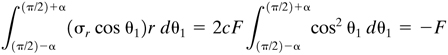
from which, after integration, c = −1/(2α − sin 2α). Thus, by replacing θ1 with 90° − θ, we have
(3.42)
![]()
It is seen that if θ1 is larger than π/2 the radial stress is positive, that is, tension exists. Because sin θ = y/r, cos θ = x/r, and ![]() , the normal and shearing stresses at a point over any cross section m − n, using Eqs. (3.34) and (3.42), may be expressed as
, the normal and shearing stresses at a point over any cross section m − n, using Eqs. (3.34) and (3.42), may be expressed as
(3.43)
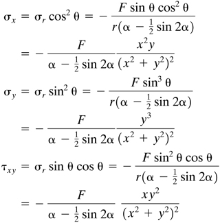
Using Eqs. (3.43), it can be shown that (Prob. 3.33) across a transverse section x = L of the wedge: σx is a maximum for θ = ±30°, σy is a maximum for θ = ±60°, and τxy is a maximum for θ = ±45°.
To compare the results given by Eqs. (3.43) with the results given by the elementary formulas for stress, consider the series
It follows that, for small angle α, we can disregard all but the first two terms of this series to obtain
(f)
![]()
By introducing the moment of inertia of the cross section m – n, ![]() · tan3α, and Eq. (f), we find from Eqs. (3.43) that
· tan3α, and Eq. (f), we find from Eqs. (3.43) that
(g)

For small values of α, the factor in the bracket is approximately equal to unity. The expression for αx then coincides with that given by the flexure formula, −My/I, of the mechanics of materials. In the elementary theory, the lateral stress σy given by the second of Eqs. (3.43) is ignored. The maximum shearing stress τxy obtained from Eq. (g) is twice as great as the shearing stress calculated from VQ/Ib of the elementary theory and occurs at the extreme fibers (at points m and n) rather than the neutral axis of the rectangular cross section.
In the case of loading in both compression and bending, superposition of the effects of P and F results in the following expression for combined stress in a pivot or in a wedge-cantilever:
(3.44)
![]()
The foregoing provides the local stresses at the support of a beam of narrow rectangular cross section.
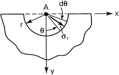
Concentrated Load on a Straight Boundary (Fig. 3.11a)
Figure 3.11. (a) Concentrated load on a straight boundary of a large plate; (b) a circle of constant radial stress.

By setting α = π/2 in Eq. (3.40), the result
(3.45)
![]()
is an expression for radial stress in a very large plate (semi-infinite solid) under normal load at its horizontal surface. For a circle of any diameter d with center on the x axis and tangent to the y axis, as shown in Fig. 3.11b, we have, for point A of the circle, d · cos θ = r. Equation (3.45) then becomes
(3.46)
![]()
We thus observe that, except for the point of load application, the stress is the same at all points on the circle.
The stress components in Cartesian coordinates may be obtained readily by following a procedure similar to that described previously for a wedge:
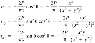
The state of stress is shown on a properly oriented element in Fig. 3.11a.
3.10 Stress Distribution Near Concentrated Load Acting on a Beam
The elastic flexure formula for beams gives satisfactory results only at some distance away from the point of load application. Near this point, however, there is a significant perturbation in stress distribution, which is very important. In the case of a beam of narrow rectangular cross section, these irregularities can be studied by using the equations developed in Sec. 3.9.
Consider the case of a simply supported beam of depth h, length L, and width b, loaded at the midspan (Fig. 3.12a). The origin of coordinates is taken to be the center of the beam, with x the axial axis as shown in the figure. Both force P and the supporting reactions are applied along lines across the width of the beam. The bending stress distribution, using the flexure formula, is expressed by

Figure 3.12. Beam subjected to a concentrated load P at the midspan.

where I = bh3/12 is the moment of inertia of the cross section. The stress at the loaded section is obtained by substituting x = 0 into the preceding equation:
(a)
![]()
To obtain the total stress along section AB, we apply the superposition of the bending stress distribution and stresses created by the line load, given by Eq. (3.45) for a semi-infinite plate. Observe that the radial pressure distribution created by a line load over quadrant ab of cylindrical surface abc at point A (Fig. 3.12b) produces a horizontal force
(b)
![]()
and a vertical force
(c)
![]()
applied at A (Fig. 3.12c). In the case of a beam (Fig. 3.12a), the latter force is balanced by the supporting reactions that give rise to the bending stresses [Eq. (a)]. On the other hand, the horizontal forces create tensile stresses at the midsection of the beam of
(d)
![]()
as well as bending stresses of
(e)
![]()
Here Ph/2π is the bending moment of forces P/π about the point 0.
Combining the stresses of Eqs. (d) and (e) with the bending stress given by Eq. (a), we obtain the axial normal stress distribution over beam cross section AB:
(3.48)
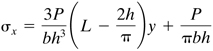
At point B(0, h/2), the tensile stress is
(3.49)
The second term represents a correction to the simple beam formula owing to the presence of the line load. It is observed that for short beams this stress is of considerable magnitude. The axial normal stresses at other points in the midsection are determined in a like manner.
The foregoing procedure leads to the poorest accuracy for point B, the point of maximum tensile stress. A better approximation [see Ref. 3.7] of this stress is given by
(3.50)
![]()
Another more detailed study demonstrates that the local stresses decrease very rapidly with increase of the distance (x) from the point of load application. At a distance equal to the depth of the beam, they are usually negligible. Furthermore, along the loaded section, the normal stress σx does not obey a linear law.
In the preceding discussion, the disturbance caused by the reactions at the ends of the beam, which are also applied as line loads, are not taken into account. To determine the radial stress distribution at the supports of the beam of narrow rectangular cross section, Eq. (3.44) can be utilized. Clearly, for the beam under consideration, we use F = 0 and replace P by P/2 in this expression.
3.11 Stress Concentration Factors
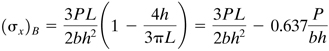
The discussion of Sec. 3.9 shows that, for situations in which the cross section of a load-carrying member varies gradually, reasonably accurate results can be expected if we apply equations derived on the basis of constant section. On the other hand, where abrupt changes in the cross section exist, the mechanics of materials approach cannot predict the high values of stress that actually exist. The condition referred to occurs in such frequently encountered configurations as holes, notches, and fillets. While the stresses in these regions can in some cases (for example, Table 3.2) be analyzed by applying the theory of elasticity, it is more usual to rely on experimental techniques and, in particular, photoelastic methods. The finite element method (Chapter 7) is very efficient for this purpose.
Table 3.2
It is to be noted that irregularities in stress distribution associated with abrupt changes in cross section are of practical importance in the design of machine elements subject to variable external forces and stress reversal. Under the action of stress reversal, progressive cracks (Sec. 4.4) are likely to start at certain points at which the stress is far above the average value. The majority of fractures in machine elements in service can be attributed to such progressive cracks.
It is usual to specify the high local stresses owing to geometrical irregularities in terms of a stress concentration factor, k. That is,
(3.51)
![]()
Clearly, the nominal stress is the stress that would exist in the section in question in the absence of the geometric feature causing the stress concentration. The technical literature contains an abundance of specialized information on stress concentration factors in the form of graphs, tables, and formulas.*
* See, for example, Refs. 3.8 through 3.11.
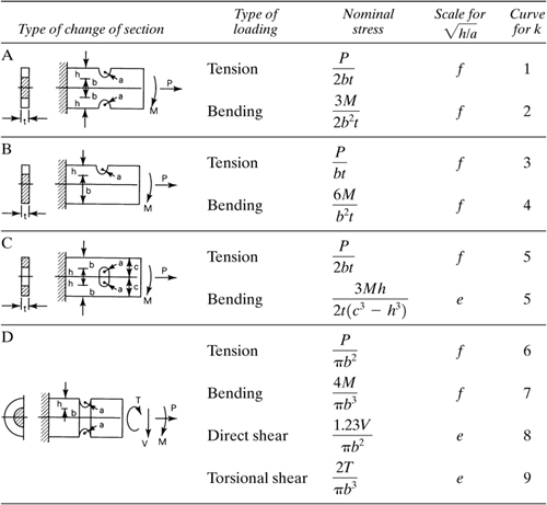
A large, thin plate containing a small circular hole of radius a is subjected to simple tension (Fig. 3.13a). Determine the field of stress and compare with those of Example 3.3.
Figure 3.13. Example 3.4. Circular hole in a plate subjected to uniaxial tension: (a) tangential stress distribution for θ = ±π/2; (b) tangential stress distribution along periphery of the hole.
Solution The boundary conditions appropriate to the circumference of the hole are
(a)
![]()
For large distances away from the origin, we set σr, σθ, and τrθ equal to the values found for a solid plate in Example 3.3. Thus, from Eq. (3.39), for r = ∞,
(b)
![]()
For this case, we assume a stress function analogous to Eq. (h) of Example 3.3,
(c)
![]()
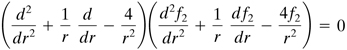
in which f1 and f2 are yet to be determined. Substituting Eq. (c) into the biharmonic equation (3.37) and noting the validity of the resulting expression for all θ, we have
(d)
(e)
The solutions of Eqs. (d) and (e) are (Prob. 3.35)
(f)
![]()
(g)
![]()
where the c’s are the constants of integration. The stress function is then obtained by introducing Eqs. (f) and (g) into (c). By substituting Φ into Eq. (3.29), the stresses are found to be
(h)
The absence of c4 indicates that it has no influence on the solution.
According to the boundary conditions (b), c1 = c6 = 0 in Eq. (h), because as r → ∞ the stresses must assume finite values. Then, according to the conditions (a), the equations (h) yield
![]()
![]()
![]()
Also, from Eqs. (b) and (h) we have
![]()
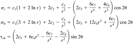
Solving the preceding five expressions, we obtain c2 = σo/4, c3 = −a2σo/2, c5 = −σ0/4, c7 = −a4σ0/4, and c8 = a2σ0/2. The determination of the stress distribution in a large plate containing a small circular hole is completed by substituting these constants into Eq. (h):
(3.25a)

(3.25b)
(3.25c)

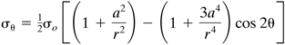
The tangential stress distribution along the edge of the hole, r = a, is shown in Fig. 3.13b using Eq. (3.52b). We observe from the figure that
![]()
The latter indicates that there exists a small area experiencing compressive stress. On the other hand, from Eq. (3.39) for θ = ±π/2, (σθ)max = σo. The stress concentration factor, defined as the ratio of the maximum stress at the hole to the nominal stress σo is therefore k = 3σo/σo = 3.
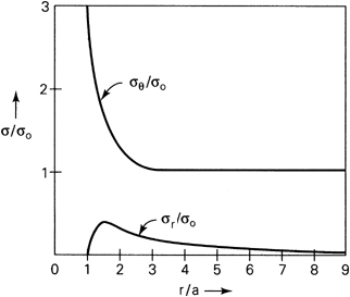
To depict the variation of σr(r, π/2) and σθ(r, π/2) over the distance from the origin, dimensionless stresses are plotted against the dimensionless radius in Fig. 3.14. The shearing stress τrθ(r, π/2) = 0. At a distance of twice the diameter of the hole, that is, r = 4a, we obtain σθ ≈ 1.037σo and σr ≈ 0.088σo. Similarly, at a distance r = 9a, we have σθ ≈ 1.006σo and σr ≈ 0.018σo, as is observed in the figure. Thus, simple tension prevails at a distance of approximately nine radii; the hole has a local effect on the distribution of stress. This is a verification of Saint-Venant’s principle.
Figure 3.14. Example 3.4. Graph of tangential and radial stresses for θ = π/2 versus the distance from the center of the plate shown in Fig. 3.13a.
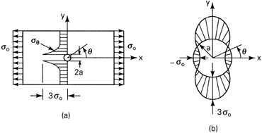
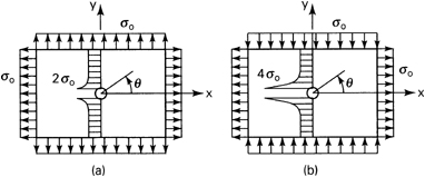
The results expressed by Eqs. (3.52) are applied, together with the method of superposition, to the case of biaxial loading. Distributions of maximum stress σθ (r, π/2), obtained in this way (Prob. 3.36), are given in Fig. 3.15. Such conditions of stress concentration occur in a thin-walled spherical pressure vessel with a small circular hole (Fig. 3.15a) and in the torsion of a thin-walled circular tube with a small circular hole (Fig. 3.15b).
Figure 3.15. Tangential stress distribution for θ = ±π/2 in the plate with the circular hole subject to biaxial stresses: (a) uniform tension; (b) pure shear.
It is noted that a similar stress concentration is caused by a small elliptical hole in a thin, large plate (Fig. 3.16). It can be shown that the maximum tensile stress at the ends of the major axis of the hole is given by
(3.53)

Figure 3.16. Elliptical hole in a plate under uniaxial tension.

Clearly, the stress increases with the ratio b/a. In the limit as a → 0, the ellipse becomes a crack of length 2b, and a very high stress concentration is produced; material will yield plastically around the ends of the crack or the crack will propagate. To prevent such spreading, holes may be drilled at the ends of the crack to effectively increase the radii to correspond to a smaller b/a. Thus, a high stress concentration is replaced by a relatively smaller one.
3.12 Neuber’s Diagram
Several geometries of practical importance, given in Table 3.2, were the subject of stress concentration determination by Neuber on the basis of mathematical analysis, as in the preceding example. Neuber’s diagram (a nomograph), which is used with the table for determining the stress concentration factor k for the configurations shown, is plotted in Fig. 3.17. In applying Neuber’s diagram, the first step is the calculation of the values of ![]() and
and ![]() .
.
Figure 3.17. Neuber’s nomograph.

Given a value of ![]() , we proceed vertically upward to cut the appropriate curve designated by the number found in column 5 of the table, then horizontally to the left to the ordinate axis. This point is then connected by a straight line to a point on the left abscissa representing
, we proceed vertically upward to cut the appropriate curve designated by the number found in column 5 of the table, then horizontally to the left to the ordinate axis. This point is then connected by a straight line to a point on the left abscissa representing ![]() , according to either scale e or f as indicated in column 4 of the table. The value of k is read off on the circular scale at a point located on a normal from the origin. [The values of (theoretical) stress concentration factors obtained from Neuber’s nomograph agree satisfactorily with those found by the photoelastic method.]
, according to either scale e or f as indicated in column 4 of the table. The value of k is read off on the circular scale at a point located on a normal from the origin. [The values of (theoretical) stress concentration factors obtained from Neuber’s nomograph agree satisfactorily with those found by the photoelastic method.]
Consider, for example, the case of a member with a single notch (Fig. B in the table), and assume that it is subjected to axial tension P only. For given a = 7.925 mm, h = 44.450 mm, and b = 266.700 mm, ![]() and
and ![]() Table 3.2 indicates that scale f and curve 3 are applicable. Then, as just described, the stress concentration factor is found to be k = 3.25. The path followed is denoted by the broken lines in the diagram. The nominal stress P/bt, multiplied by k, yields maximum theoretical stress, found at the root of the notch.
Table 3.2 indicates that scale f and curve 3 are applicable. Then, as just described, the stress concentration factor is found to be k = 3.25. The path followed is denoted by the broken lines in the diagram. The nominal stress P/bt, multiplied by k, yields maximum theoretical stress, found at the root of the notch.
Example 3.5
A circular shaft with a circumferential circular groove (notch) is subjected to axial force P, bending moment M, and torque T (Fig. D of Table 3.2). Determine the maximum principal stress.
Solution For the loading described, the principal stresses occur at a point at the root of the notch which, from Eq. (1.16), are given by
(a)
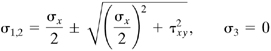
where σx and τxy represent the normal and shear stresses in the reduced cross section of the shaft, respectively. We have
![]()
or
(b)
![]()
Here ka, kb, and kt denote the stress concentration factors for axial force, bending moment, and torque, respectively. These factors are determined from curves 6, 7, and 9 in Fig. 3.17. Thus, given a set of shaft dimensions and the loading, formulas (a) and (b) lead to the value of the maximum principal stress σ1.
In addition, note that a shear force V may also act on the shaft (as in Fig. D of Table 3.2). For slender members, however, this shear contributes very little to the deflection (Sec. 5.4) and to the maximum stress.
3.13 Contact Stresses
Application of a load over a small area of contact results in unusually high stresses. Situations of this nature are found on a microscopic scale whenever force is transmitted through bodies in contact. There are important practical cases when the geometry of the contacting bodies results in large stresses, disregarding the stresses associated with the asperities found on any nominally smooth surface. The Hertz problem relates to the stresses owing to the contact of a sphere on a plane, a sphere on a sphere, a cylinder on a cylinder, and the like. The practical implications with respect to ball and roller bearings, locomotive wheels, valve tappets, and numerous machine components are apparent.
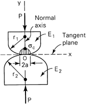
Consider, in this regard, the contact without deformation of two bodies having spherical surfaces of radii r1 and r2, in the vicinity of contact. If now a collinear pair of forces P acts to press the bodies together, as in Fig. 3.18, deformation will occur, and the point of contact O will be replaced by a small area of contact. A common tangent plane and common normal axis are denoted Ox and Oy, respectively. The first steps taken toward the solution of this problem are the determination of the size and shape of the contact area as well as the distribution of normal pressure acting on the area. The stresses and deformations resulting from the interfacial pressure are then evaluated.
Figure 3.18. Spherical surfaces of two bodies compressed by forces P.
The following assumptions are generally made in the solution of the contact problem:
1. The contacting bodies are isotropic and elastic.
2. The contact areas are essentially flat and small relative to the radii of curvature of the undeformed bodies in the vicinity of the interface.
3. The contacting bodies are perfectly smooth, and therefore only normal pressures need be taken into account.
The foregoing set of assumptions enables an elastic analysis to be conducted. Without going into the derivations, we shall, in the following paragraphs, introduce some of the results.* It is important to note that, in all instances, the contact pressure varies from zero at the side of the contact area to a maximum value σc at its center.
* A summary and complete list of references dealing with contact stress problems are given by Refs. 3.12 through 3.16.
Two Spherical Surfaces in Contact
Because of forces P (Fig. 3.18), the contact pressure is distributed over a small circle of radius a given by
(3.54)
![]()
where E1 and E2 (r1 and r2) are the respective moduli of elasticity (radii) of the spheres. The force P causing the contact pressure acts in the direction of the normal axis, perpendicular to the tangent plane passing through the contact area. The maximum contact pressure is found to be
(3.55)
![]()
This is the maximum principal stress owing to the fact that, at the center of the contact area, material is compressed not only in the normal direction but also in the lateral directions. The relationship between the force of contact P, and the relative displacement of the centers of the two elastic spheres, owing to local deformation, is
(3.56)
![]()
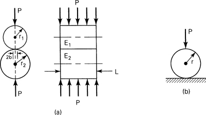
In the special case of a sphere of radius r contacting a body of the same material but having a flat surface (Fig. 3.19a), substitution of r1 = r, r2 = ∞, and E1 = E2 = E into Eqs. (3.54) through (3.56) leads to
(3.57)
![]()
Figure 3.19. Contact load: (a) in sphere on a plane; (b) in ball in a spherical seat.
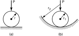
For the case of a sphere in a spherical seat of the same material (Fig. 3.19b) substituting r2 = –r2 and E1 = E2 = E in Eqs. (3.54) through (3.56), we obtain
(3.58)

Two Parallel Cylindrical Rollers
Here the contact area is a narrow rectangle of width 2b and length L (Fig. 3.20a). The maximum contact pressure is given by
(3.59)
![]()
Figure 3.20. Contact load: (a) in two cylindrical rollers; (b) in cylinder on a plane.
where
(3.60)
![]()
In this expression, Ei(vi) and ri, with i = 1, 2, are the moduli of elasticity (Poisson’s ratio) of the two rollers and the corresponding radii, respectively. If the cylinders have the same elastic modulus E and Poisson’s ratio v = 0.3, these expressions reduce to
(3.61)
![]()
Figure 3.20b shows the special case of contact between a circular cylinder of radius r and a flat surface, both bodies of the same material. After rearranging the terms and taking r1 = r and r2 = ∞ in Eqs. (3.61), we have
(3.62)
![]()
Two Curved Surfaces of Different Radii
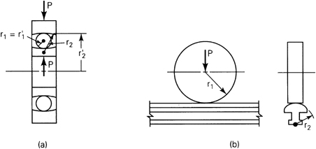
Consider now two rigid bodies of equal elastic moduli E, compressed by force P (Fig. 3.21). The load lies along the axis passing through the centers of the bodies and through the point of contact and is perpendicular to the plane tangent to both bodies at the point of contact. The minimum and maximum radii of curvature of the surface of the upper body are r1 and r’1; those of the lower body are r2 and ![]() at the point of contact. Thus,
at the point of contact. Thus, ![]() are the principal curvatures. The sign convention of the curvature is such that it is positive if the corresponding center of curvature is inside the body. If the center of the curvature is outside the body, the curvature is negative. (For example, in Fig. 3.22a, r1
are the principal curvatures. The sign convention of the curvature is such that it is positive if the corresponding center of curvature is inside the body. If the center of the curvature is outside the body, the curvature is negative. (For example, in Fig. 3.22a, r1![]() are positive, while r2,
are positive, while r2, ![]() are negative.)
are negative.)
Figure 3.21. Curved surfaces of different radii of two bodies compressed by forces P.

Figure 3.22. Contact load: (a) in a single-row ball bearing; (b) in a cylindrical wheel and rail.
Let θ be the angle between the normal planes in which radii r1 and r2 lie. Subsequent to loading, the area of contact will be an ellipse with semiaxes a and b (Table C.1). The maximum contact pressure is
(3.63)
![]()
In this expression the semiaxes are given by
(3.64)
![]()
Here
(3.65)
The constants ca and cb are read in Table 3.3. The first column of the table lists values of α, calculated from
(3.66)
![]()
Table 3.3
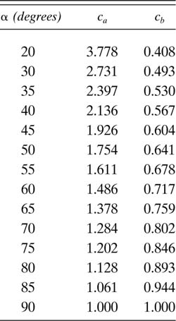
(3.67)

By applying Eq. (3.63), many problems of practical importance may be treated, for example, contact stresses in ball bearings (Fig. 3.22a), contact stresses between a cylindrical wheel and a rail (Fig. 3.22b), and contact stresses in cam and push-rod mechanisms.
A railway car wheel rolls on a rail. Both rail and wheel are made of steel for which E = 210 GPa and ν = 0.3. The wheel has a radius of r1 = 0.4 m, and the cross radius of the rail top surface is r2 = 0.3 m (Fig. 3.22b). Determine the size of the contact area and the maximum contact pressure, given a compression load of P = 90 kN.
Solution For the situation described, ![]() and, because the axes of the members are mutually perpendicular, θ = π/2. The first of Eqs. (3.65) and Eqs. (3.67) reduce to
and, because the axes of the members are mutually perpendicular, θ = π/2. The first of Eqs. (3.65) and Eqs. (3.67) reduce to
(3.68)
![]()
The proper sign in B must be chosen so that its values are positive. Now Eq. (3.66) has the form
(3.69)
![]()
Substituting the given numerical values into Eqs. (3.68), (3.69), and the second of (3.65), we obtain
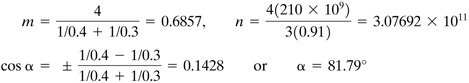
Corresponding to this value of α, interpolating in Table 3.3, we have
![]()
The semiaxes of the elliptical contact are found by applying Eqs. (3.64):

The maximum contact pressure, or maximum principal stress, is thus
![]()
A hardened steel material is capable of resisting this or somewhat higher stress levels for the body geometries and loading conditions described in this section.
Problems
Secs. 3.1 through 3.7
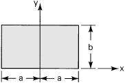
3.1. A stress distribution is given by
(a)
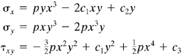
where the p and c’s are constants. (a) Verify that this field represents a solution for a thin plate of thickness t (Fig. P3.1); (b) obtain the corresponding stress function; (c) find the resultant normal and shearing boundary forces (Py and Vx) along edges y = 0 and y = b of the plate.
Figure P3.1.
3.2. If the stress field given by Eq. (a) of Prob. 3.1 acts in the thin plate shown in Fig. P3.1 and p is a known constant, determine the c’s so that edges x = ±a are free of shearing stress and no normal stress acts on edge x = a.
3.3. In bending of a rectangular plate (Fig. P3.3), the state of stress is expressed by
Figure P3.3.

![]()
(a) What conditions among the constants (the c’s) make the preceding expressions possible? Body forces may be neglected. (b) Draw a sketch showing the boundary stresses on the plate.
3.4. Given the following stress field within a structural member,

where a and b are constants. Determine whether this stress distribution represents a solution for a plane strain problem. The body forces are omitted.
3.5. Determine whether the following stress functions satisfy the conditions of compatibility for a two-dimensional problem:
(a)
![]()
(b)
![]()
Here a, b, c, and d are constants. Also obtain the stress fields that arise from Φ1 and Φ2.
3.6. Figure P3.6 shows a long, thin steel plate of thickness t, width 2h, and length 2a. The plate is subjected to loads that produce the uniform stresses σo at the ends. The edges at y = ±h are placed between the two rigid walls. Show that, by using an inverse method, the displacements are expressed by
Figure P3.6.

![]()
3.7. Determine whether the following stress distribution is a valid solution for a two-dimensional problem:
![]()
where a is a constant. Body forces may be neglected.
3.8. The strain distribution in a thin plate has the form
![]()
in which a is a small constant. Show whether this strain field is a valid solution of an elasticity problem. Body forces may be disregarded.
3.9. The components of the displacement of a thin plate (Fig. P3.9) are given by
![]()
Figure P3.9.

Here c is a constant and ν represents Poisson’s ratio. Determine the stresses σx, σy, and τxy. Draw a sketch showing the boundary stresses on the plate.
3.10. Consider a rectangular plate with sides a and b of thickness t (Fig. P3.10). (a) Determine the stresses σx, σy, and τxy for the stress function Φ = px3y, where p is a constant. (b) Draw a sketch showing the boundary stresses on the plate. (c) Find the resultant normal and shearing boundary forces (Px, Py, Vx, and Vy) along all edges of the plate.
Figure P3.10.

3.11. Redo Prob. 3.10 for the case of a square plate of side dimensions a and
![]()
where p is a constant.
3.12. Resolve Prob. 3.10 a and b for the stress function of the form
![]()
where p represents a constant.
3.13. A vertical force P per unit thickness is applied on the horizontal boundary of a semi-infinite solid plate of unit thickness (Fig. 3.11a). Show that the stress function Φ = −(P/π)y tan−1(y/x) results in the following stress field within the plate:
![]()
Also plot the resulting stress distribution for σx and τxy at a constant depth L below the boundary.
3.14. The thin cantilever shown in Fig. P3.14 is subjected to uniform shearing stress τo along its upper surface (y = +h) while surfaces y = −h and x = L are free of stress. Determine whether the Airy stress function
Figure P3.14.

satisfies the required conditions for this problem.
3.15. Figure P3.15 shows a thin cantilever beam of unit thickness carrying a uniform load of intensity p per unit length. Assume that the stress function is expressed by
Φ = ax2 + bx2y + cy3 + dy5 + ex2y3
Figure P3.15.

in which a, …, e are constants. Determine (a) the requirements on a, …, e so that Φ is biharmonic; (b) the stresses σx, σy, and τxy.
3.16. Consider a thin square plate with sides a. For a stress function ![]() , determine the stress field and sketch it along the boundaries of the plate. Here p represents a uniformly distributed loading per unit length. Note that the origin of the x, y coordinate system is located at the lower-left corner of the plate.
, determine the stress field and sketch it along the boundaries of the plate. Here p represents a uniformly distributed loading per unit length. Note that the origin of the x, y coordinate system is located at the lower-left corner of the plate.
3.17. Consider a thin cantilever loaded as shown in Fig. P3.17. Assume that the bending stress is given by
(P3.17)
![]()
Figure P3.17.

and σz = τxz = τyz = 0. Determine the stress components σy and τxy as functions of x and y.
3.18. Show that for the case of plane stress, in the absence of body forces, the equations of equilibrium may be expressed in terms of displacements u and υ as follows:
(P3.18)
[Hint: Substitute Eqs. (3.10) together with (2.3) into (3.6).]
3.19. Determine whether the following compatible stress field is possible within an elastic uniformly loaded cantilever beam (Fig. P3.17):
Here I = 2th3/3 and the body forces are omitted. Given p = 10 kN/m, L = 2 m, h = 100 mm, t = 40 mm, ν = 0.3, and E = 200 GPa, calculate the magnitude and direction of the maximum principal strain at point Q.
3.20. A prismatic bar is restrained in the x (axial) and y directions, but free to expand in z direction. Determine the stresses and strains in the bar for a temperature rise of T1 degrees.
3.21. Under free thermal expansion, the strain components within a given elastic solid are εx = εy = εz = αT and γxy = γyz = γxz = 0. Show that the temperature field associated with this condition is of the form
α T = c1x + c2y + c3z + c4
in which the c’s are constants.
3.22. Redo Prob. 3.6 adding a temperature change T1, with all other conditions remaining unchanged.
3.23. Determine the axial force Px and moment Mz that the walls in Fig. 3.6b apply to the beam for T = a1y + a2, where a1 and a2 are constant.
3.24. A copper tube of 800-mm2 cross-sectional area is held at both ends as in Fig. P3.24. If at 20°C no axial force Px exists in the tube, what will Px be when the temperature rises to 120°C? Let E = 120 GPa and α = 16.8 × 10⁻⁶per °C.
Figure P3.24.
3.25. Show that the case of a concentrated load on a straight boundary (Fig. 3.11a) is represented by the stress function
![]()
and derive Eqs. (3.45) from the result.
3.26. Verify that Eqs. (3.34) are determined from the equilibrium of forces acting on the elements shown in Fig. P3.26.
Figure P3.26.
3.27. Demonstrate that the biharmonic equation ∇4Φ = 0 in polar coordinates can be written as

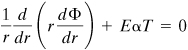
3.28. Show that the compatibility equation in polar coordinates, for the axisymmetrical problem of thermal elasticity, is given by
(P3.28)
3.29. Assume that moment M acts in the plane and at the vertex of the wedge-cantilever shown in Fig. P3.29. Given a stress function
(P3.29a)
![]()
Figure P3.29.
determine (a) whether Φ satisfies the condition of compatibility; (b) the stress components σr, σθ, and τrθ; and (c) whether the expressions
(P3.29b)
![]()
represent the stress field in a semi-infinite plate (that is, for α = π/2).
3.30. Referring to Fig. P3.30, verify the results given by Eqs. (b) and (c) of Sec. 3.10.
Figure P3.30.
3.31. Consider the pivot of unit thickness subject to force P per unit thickness at its vertex (Fig. 3.10a). Determine the maximum values of σx and τxy on a plane a distance L from the apex through the use of σr given by Eq. (3.40) and the formulas of the elementary theory: (a) take α = 15°; (b) take α = 60°. Compare the results given by the two approaches.
3.32. Solve Prob. 3.31 for α = 30°.
3.33. Redo Prob. 3.31 in its entirety for the wedge-cantilever shown in Fig. 3.10b.
3.34. A uniformly distributed load of intensity p is applied over a short distance on the straight edge of a large plate (Fig. P3.34). Determine stresses σx, σy, and τxy in terms of p, θ1, and θ2, as required. [Hint: Let dP = pdy denote the load acting on an infinitesimal length dy = rd θ/cos θ (from geometry) and hence dP = prd θ/cos θ. Substitute this into Eqs. (3.47) and integrate the resulting expressions.]
Figure P3.34.

Secs. 3.11 through 3.13
3.35. Verify the result given by Eqs. (f) and (g) of Sec. 3.11 (a) by rewriting Eqs. (d) and (e) in the following forms, respectively,
(P3.35)

and by integrating (P3.35) and (b) by expanding Eqs. (d) and (e), setting t = In r, and thereby transforming the resulting expressions into two ordinary differential equations with constant coefficients.
3.36. Verify the results given in Fig. 3.15 by employing Eq. (3.52b) and the method of superposition.
3.37. For the flat bar of Fig. C of Table 3.2, let b = 17h, c = 18h, and a = h (circular hole). Referring to Neuber’s nomograph (Fig. 3.17), determine the value of k for the bar loaded in tension.
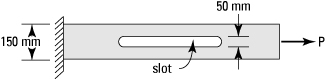
3.38. A 20-mm-thick steel bar with a slot (25 mm radii at ends) is subjected to an axial load P, as shown in Fig. P3.38. What is the maximum stress for P = 180 kN?
Figure P3.38.
3.39. For the flat bar in Fig. A of Table 3.2, let h = 3a and b = 15a. Referring to Neuber’s nomograph (Fig. 3.17), find the value of k for the bar subjected to (a) axial tensile load, and (b) bending.
3.40. A thin-walled circular cylindrical vessel of diameter d and wall thickness t is subjected to internal pressure p (see Table 1.1). Given a small circular hole in the vessel wall, show that the maximum tangential and axial stresses at the hole are σθ = 5pd/4t and σa = pd/4t, respectively.
3.41. The shaft shown in Fig. D of Table 3.2 has the following dimensions: a = 6 mm, h = 12 mm, and b = 200 mm. The shaft is subjected simultaneously to a torque T = 4 kN . m, a bending moment M = 2 kN . m, and an axial force P = 10 kN. Calculate at the root of the notch (a) the maximum principal stress, (b) the maximum shear stress, and (c) the octahedral stresses.
3.42. Redo Prob. 3.41 for a = 4 mm, h = 6 mm, b = 120 mm, T = 3 kN·m, M = 1.5kN·m, and P = 0.
3.43. A 50-mm-diameter ball is pressed into a spherical seat of diameter 75 mm by a force of 500 N. The material is steel (E = 200 GPa, ν = 0.3). Calculate (a) the radius of the contact area; (b) the maximum contact pressure; and (c) the relative displacement of the centers of the ball and seat.
3.44. Calculate the maximum contact pressure σc in Prob. 3.43 for the cases when the 50-mm-diameter ball is pressed against (a) a flat surface, and (b) an identical ball.
3.45. Calculate the maximum pressure between a steel wheel of radius r1 = 400 mm and a steel rail of crown radius of the head r2 = 250 mm (Fig. 3.22b) for P = 4 kN. Use E = 200 GPa and ν = 0.3.
3.46. A concentrated load of 2.5 kN at the center of a deep steel beam is applied through a 10-mm-diameter steel rod laid across the 100-mm beam width. Compute the maximum contact pressure and the width of the contact between rod and beam surface. Use E = 200 GPa and ν = 0.3.
3.47. Two identical 400-mm-diameter steel rollers of a rolling mill are pressed together with a force of 2 MN/m. Using E = 200 GPa and ν = 0.25, compute the maximum contact pressure and width of contact.
3.48. Determine the size of the contact area and the maximum pressure between two circular cylinders with mutually perpendicular axes. Denote by r1 and r2 the radii of the cylinders. Use r1 = 500 mm, r2 = 200 mm, P = 5 kN, E = 210 GPa, and ν = 0.25.
3.49. Solve Prob. 3.48 for the case of two cylinders of equal radii, r1 = r2 = 200 mm.
3.50. Determine the maximum pressure at the contact point between the outer race and a ball in the single-row ball bearing assembly shown in Fig. 3.22a. The ball diameter is 50 mm; the radius of the grooves, 30 mm; the diameter of the outer race, 250 mm; and the highest compressive force on the ball, P = 1.8 kN. Take E = 200 GPa and ν = 0.3.
3.51. Redo Prob. 3.50 for a ball diameter of 40 mm and a groove radius of 22 mm. Assume the remaining data to be unchanged.