
Wind Power Fundamentals
Alexander Kalmikov, Massachusetts Institute of Technology, Cambridge, MA, United States Email: [email protected]
Abstract
Wind energy technology is based on the ability to capture the energy contained in air motion. Wind power quantifies the rate of this kinetic energy extraction. Wind power is also the rate of kinetic energy flow carried by the moving air. Because the motion is both the source of the energy and the means of its transport, the efficiency of wind power extraction is a balance of slowing down the wind while maintaining a sufficient flow. This chapter quantifies these fundamental concepts and discusses the nature of wind.
Keywords
Wind energy flow rate; kinetic energy flux; wind power density; power coefficient; Betz Limit; capacity factor; source of wind energy
2.1 Wind Physics Basics: What Is Wind and How Wind Is Generated
Wind is atmospheric air in motion. It is ubiquitous and one of the basic physical elements of our environment. Depending on the speed of the moving air, wind might feel light and ethereal, being silent and invisible to the naked eye. Or, it can be a strong and destructive force, loud, and visible as a result of the heavy debris it carries along. The velocity of the air motion defines the strength of wind and is directly related to the amount of energy in the wind, i.e., its kinetic energy. The source of this energy, however, is solar radiation. The electromagnetic radiation from the Sun unevenly heats the Earth surface, stronger in the tropics and weaker in the high latitudes. Also, as a result of a differential absorption of sunlight by soil, rock, water, and vegetation, air in different regions warms up at different rate. This uneven heating is converted through convective processes to air motion, which is adjusted by the rotation of the Earth. The convective processes are disturbance of the hydrostatic balance whereby otherwise stagnant air masses are displaced and move in reaction to forces induced by changes in air density and buoyancy due to temperature differences. Air is pushed from high- to low-pressure regions, balancing friction and inertial forces due to the rotation of the Earth.
The patterns of differential Earth surface heating as well as other thermal processes such as evaporation, precipitation, clouds, shade, and variations of surface radiation absorption appear on different space and time scales. These are coupled with dynamical forces due to Earth rotation and flow momentum redistribution to drive a variety of wind generation processes, leading to the existence of a large variety of wind phenomena. These winds can be categorized based on their spatial scale and physical generation mechanisms.
2.2 Wind Types: Brief Overview of Wind Power Meteorology
Wind systems span a wide range of spatial scales, from global circulation on the planetary scale, through synoptic scale weather systems, to mesoscale regional and microscale local winds. Table 2.1 lists the spatial scales of these broad wind type categories. Examples of planetary circulations are sustained zonal flows such as the jet stream, trade winds, and polar jets. Mesoscale winds include orographic and thermally induced circulations [1]. On the microscale wind systems include flow channeling by urban topography [2] as well as submesoscale convective wind storm phenomena as an example.
Table 2.1
Spatial Scales of Wind Systems and a Sample of Associated Wind Types
| Spatial Scales | Wind Types | Length Scale |
| Planetary scale | Global circulation | 10, 000 km |
| Synoptic scale | Weather systems | 1000 km |
| Mesoscale | Regional orographic or thermally induced circulations | 10–100 km |
| Microscale | Local flow modulation, boundary layer turbulent gusts | 100–1000 m |
A long list of various wind types can be assembled from scientific and colloquial names of different winds around the world. The associated physical phenomena enable a finer classification across the spatial scales. Generating physical mechanisms define geostrophic winds, thermal winds, and gradient winds. Katabatic and anabatic winds are local topographic winds generated by cooling and heating of mountain slopes. Bora, Foehn, and Chinook are locale specific names for strong downslope wind storms [3]. In Greenland, Piteraq is a downslope storm as strong as a hurricane, with sustained wind speeds of 70 m s−1 (160 miles per hour). In coastal areas sea breeze and land breeze circulations are regular daily occurrences. Convective storms generate strong transient winds, with downdrafts which can be particularly dangerous (and not very useful for wind power harvesting). Disastrous hurricanes and typhoons, as well as smaller scale tornadoes, are examples of very energetic and destructive wind systems. A microscale version of these winds is gusts, dust devils, and microbursts. Nocturnal jets appear in regular cycles in regions with specific vertical atmospheric structure. Atmospheric waves driven by gravity and modulated by topography are common in many places. Locale specific regional wind names include Santa Anas, nor’easters, and etesian winds, to mention just few.
Meteorology is the scientific field involved in the study and explanation of all these wind phenomena. It enables both a theoretical understanding and the practical forecasting capabilities of wind capabilities. Statistics of observed wind occurrences define wind climates in different regions. Mathematical and computer models are used for theoretical simulation, exploratory resource assessment, and operational forecasting of winds. Meteorology literature focusing on wind power is available in the form of introductory texts and reviews [4–7].
2.3 Fundamental Equation of Wind Power: Kinetic Energy Flux and Wind Power Density
The fundamental equation of wind power answers the most basic quantitative question—how much energy is in the wind. First we distinguish between concepts of power and energy. Power is the time-rate of energy. For example, we will need to know how much energy can be generated by a wind turbine per unit time. On a more homely front, the power of the wind is the rate of wind energy flow through an open window.
• amount of air (the volume of air in consideration),
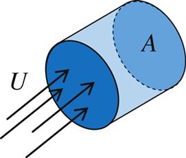
Wind power quantifies the amount of wind energy flowing through an area of interest per unit time. In other words, wind power is the flux of wind energy through an area of interest. Flux is a fundamental concept in fluid mechanics, measuring the rate of flow of any quantity carried with the moving fluid, by definition normalized per unit area. For example, mass flux is the rate of mass flow through an area of interest divided by this area. Volume flux is the volume flowing through area of interest per unit time and per unit area. Consider an area element A (Fig. 2.1) and flow of magnitude U through this area. (Here we restrict the discussion to flow perpendicular to the area of interest. In general, flow is a vector quantify that can be oriented in any direction and only its component perpendicular to the area element is considered when quantifying the flux through that area.) The volume of air flowing through this area during unit time dt is given by the volume of the cylinder with cross section area A and length ![]() , i.e., the volume
, i.e., the volume ![]() . Therefore volume flow rate is
. Therefore volume flow rate is ![]() , the volume flux is
, the volume flux is ![]() . The mass flow rate is derived by multiplying the volume flow rate by the density of the flow
. The mass flow rate is derived by multiplying the volume flow rate by the density of the flow ![]() and is equal to the mass of that cylinder divided by unit time
and is equal to the mass of that cylinder divided by unit time
(2.1)
Wind energy by definition is the energy content of air flow due to its motion. This type of energy is called the kinetic energy and is a function of fluid’s mass and velocity, given by
(2.2)
Wind power is the rate of kinetic energy flow. In derivation similar to the other flow rate quantities discussed earlier, the amount of kinetic energy flowing per unit time through a given area is equal to the kinetic energy content of the cylinder in Fig. 2.1.
(2.3)
Here mass flow rate (2.1) was substituted for air mass in Eq. (2.2). The resultant equation for wind power is
(2.4)
This is a fundamental equation in wind power analysis. It exhibits a highly nonlinear cubic dependence on wind speed. Whereby doubling the wind speed leads to eightfold increase in its available power. This explains why ambient wind speed is the major factor in considering wind energy. In Eq. (2.4), the power of the wind is a linear function of air density and as a result of the limited range of air density fluctuations, the density is of secondary importance. The power dependence on the area implies a nonlinear quadratic dependence on the radius of a wind turbine swept area, highlighting the advantages of longer wind turbine blades.
It is customary to normalize ambient wind power dividing by the area of interest; i.e., in terms of specific power flow. This leads to the definition of kinetic wind energy flux, known as the wind power density (WPD). Similarly to the definitions of flux and flow rate above, wind energy flux is wind energy flow rate per unit area is given by:
(2.5)
WPD is used to compare wind resources independent of wind turbine size and is the quantitative basis for the standard classification [8] of wind resource at the National Renewable Energy Laboratory (NREL) of the United States. Mean WPD has advantages over mean wind speed for comparing sites with different probability distribution skewness, because of the cubic nonlinear dependence of wind power on wind speed (see Fig. 11 in Ref. [9] and discussion therein). Further technical details of this classification system were originally introduced in Ref. [10]. Typical values of wind power classes with the corresponding power densities and mean wind speeds are presented in Table 2.2.
Table 2.2
Wind Power Classes Measured at 50 m Above Ground According to NREL Wind Power Density-Based Classification
| Wind Power Classification | |||
| Wind Power Class | Resource Potential | Wind Power Density/W m−2 | Wind Speed/m s−1 |
| 1 | Poor | 0–200 | 0.0–5.9 |
| 2 | Marginal | 200–300 | 5.9–6.7 |
| 3 | Fair | 300–400 | 6.7–7.4 |
| 4 | Good | 500–600 | 7.4–7.9 |
| 5 | Excellent | 500–600 | 7.9–8.4 |
| 6 | Outstanding | 600–800 | 8.4–9.3 |
| 7 | Superb | >800 | >9.3 |
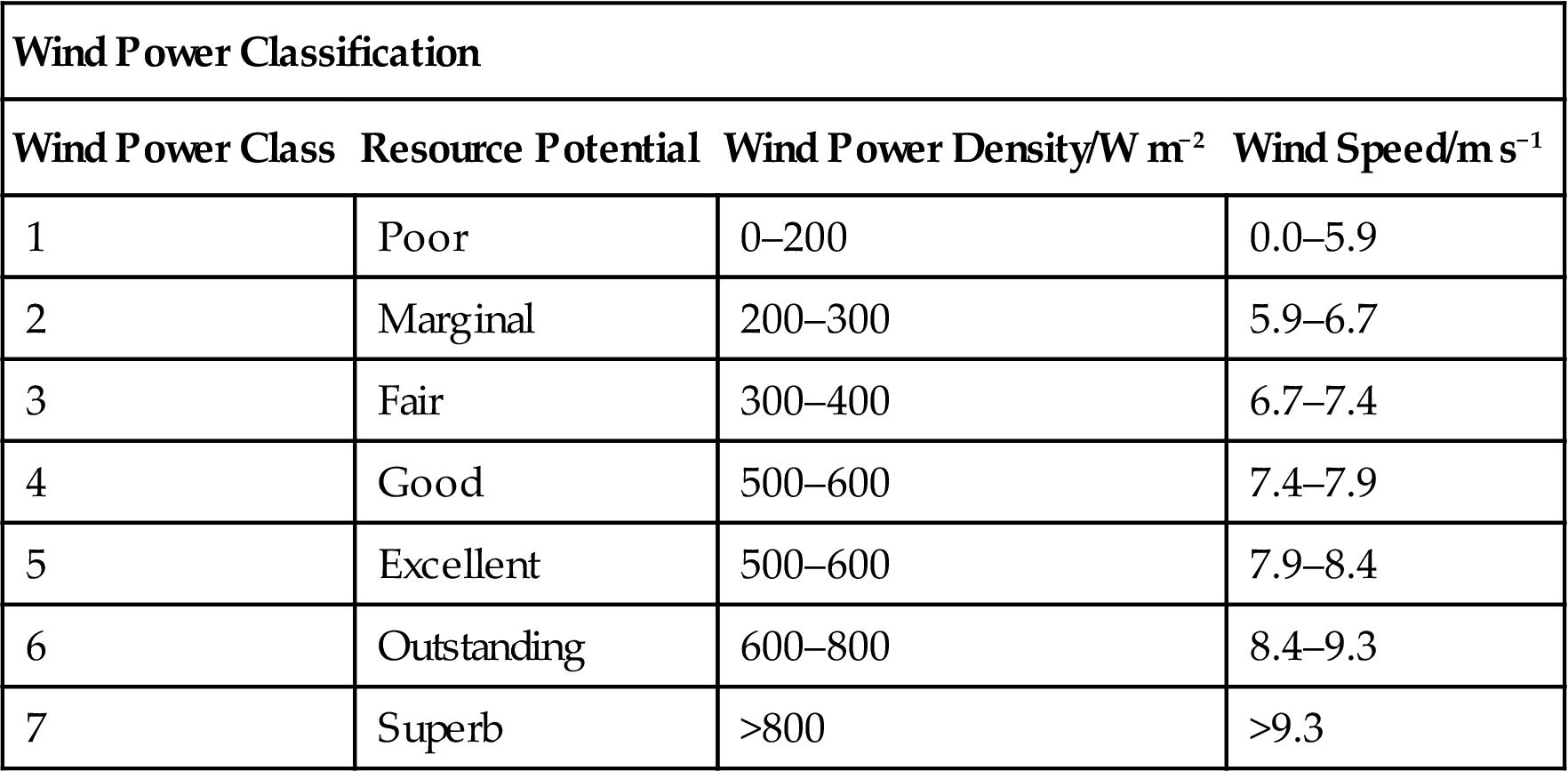
Wind speed corresponding to each class is the mean wind speed based on Rayleigh probability distribution of equivalent mean wind power density at 1500 m elevation above sea level.
Source: Data adopted from http://www.nrel.gov/gis/data/GIS_Data_Technology_Specific/United_States/Wind/50m/Colorado_Wind_50m.zip [11].
2.4 Wind Power Capture: Efficiency in Extracting Wind Power
In Section 2.3 we considered the total wind power content of ambient air flow. Fundamentally, not all this power is available for utilization. The efficiency in wind power extraction is quantified by the Power Coefficient (Cp), which is the ratio of power extracted by the turbine to the total power of the wind resource Cp=PT/Pwind.
Turbine power capture therefore is given by
(2.6)
which is always smaller than Pwind. In fact, there exists a theoretical upper limit on the maximum extractable power fraction—known as the Betz Limit. According to Betz theory [12] the maximum possible power coefficient is Cp=16/27, i.e. 59% efficiency is the best a conventional wind turbine can do in extracting power from the wind. The reason why higher, e.g., 100%, efficiency is not possible is due to the fluid mechanical nature of wind power, dependent on the continuous flow of air in motion. If, hypothetically speaking, 100% of kinetic energy was extracted then the flow of air would be reduced to a complete stop and no velocity would remain available to sustain the flow through the extraction mechanism, irrespective of the specific wind turbine technology used. The maximum extraction efficiency is achieved at the optimum balance of the largest wind slowdown that still maintains sufficiently fast flow past the turbine. (See Refs. [13,14] for further technical details and an historic account of Betz limit derivations by contemporary researchers.)
Another key metric of wind power efficiency is the Capacity Factor (CF) quantifying the fraction of the installed generating capacity that actually generates power.
(2.7)
The CF is the ratio of the actual generated energy to the energy which could potentially be generated by the system in consideration under ideal environmental conditions. Considering that energy is the product of its time-rate, i.e., the power with the elapsed time, this energy ratio is equal the ratio of average power ![]() to the nominal power of the system
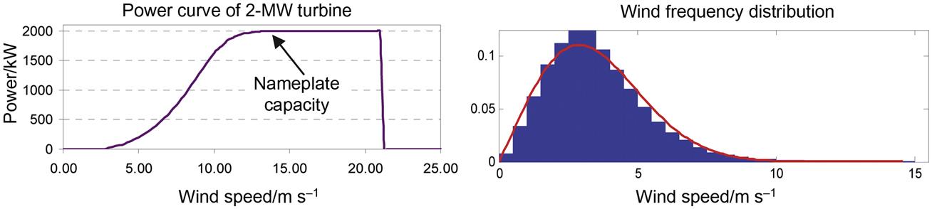
to the nominal power of the system ![]() . For a single wind turbine this nominal power is equal to its nameplate capacity, typically the maximum power it can generate under favorable wind conditions. Considering a typical power curve for a turbine (Fig. 2.2) this is the flat region for strong wind just below the cut-out wind speed.
. For a single wind turbine this nominal power is equal to its nameplate capacity, typically the maximum power it can generate under favorable wind conditions. Considering a typical power curve for a turbine (Fig. 2.2) this is the flat region for strong wind just below the cut-out wind speed.
Equivalently, CF can be regarded as the fraction of the year the turbine generator is operating at rated power (nominal capacity), i.e., the fraction of the effective time relative to the total time
(2.8)
Therefore total annual energy generation can be calculated by multiplying turbine (or wind plant) rated power ![]() by time length of 1 year and by CF.
by time length of 1 year and by CF.
(2.9)
A typical value of CF for an economically viable project is 30%, reaching about 50% in regions with a very good wind resource. The CF is based on both the characteristics of the turbine and the site—integrating the power curve with the wind resource variability (Fig. 2.2) produces the actual generation or the average power. This highlights the dependence of power production on wind variability and the importance of wind meteorology and climatology for wind power forecasting and resource assessment.
2.5 Conclusion
Wind power is concerned with the utilization of kinetic wind energy. This is the energy contained in air motion itself. Since this is a form of mechanical energy of a moving fluid, its quantification requires elements of fluid mechanics. We reviewed the concepts of kinetic energy flux and derived the fundamental equation of wind power—quantifying the rate of wind energy flow. Standard metrics of wind power resource and utilization efficiency were introduced. The nature of wind was discussed with a brief overview of wind power meteorology.