
CHAPTER
2
Moving Data Around the Oracle Environment
Data is the lifeblood of the modern organization. Much of that data is stored inside an Oracle database. As corporations merge or pursue a “best of breed” approach, IT organizations find themselves with many different repositories of data. Some data could be on legacy mainframes, financial data could be on an Oracle OLTP system, other data could be in a data warehouse, and even more could be in Big Data reservoirs or even flat files on the operating system. Making the best use of that data is the key to an efficient business plan. Often that means that data must be moved from one Oracle database to another Oracle database in a different location. It could also mean moving data from an Oracle database into a different vendor’s database. The data might have to change form from inside a database to some file outside of the database, or vice versa. There may be times when you need some of the information in the OLTP database, some historical data from the data warehouse, and still more from a legacy mainframe.
Consider the reasons why you need to move data. You may have to move it off of the OLTP system to a reporting database, or move it to a data warehouse. It might be yesterday’s sales information that needs to be shipped to a different database used by another group, or it might be a subset of financial data that is used by another department. Some of the data will need to be moved one time, other data might have to be moved on a regular basis—be it monthly or weekly or even daily. And yet more data might have to be refreshed in real time. The volume, the timeliness at which the data is needed, and even the type of data will all have to be taken into account when you are moving the data around the IT ecosystem.
There are a myriad of ways to move data within, without, and around the Oracle database. This chapter explores the many different ways in which data can flow around Oracle. Most are very familiar with the language of the database, SQL (Structured Query Language), and with Oracle’s programing language, PL/SQL. We will also talk about the old workhorse SQL*Loader. Also, some more exotic features of the Oracle database, such as external tables, can be extremely useful in moving data. What’s more, two SQL*Plus commands—SPOOL and COPY—are useful. Depending on your exact needs, each of the tools, methods, and utilities mentioned has different benefits and drawbacks. This chapter is not meant to teach you everything about these tools, but is merely an introduction so that you can explore them in depth as the occasion arises.
We will explore some of the more advanced features of moving data in a “streaming” fashion between different databases such as Streams, Oracle GoldenGate, and Advanced Replication in Chapters 3 and 4.
Structured Query Language
The most common method you will use to get data from your Oracle database is via the Structure Query Language, or SQL (pronounced sequel), the cornerstone of relational database management systems (RDBMSs). Although SQL was developed by IBM, Oracle was the first commercial implementation of SQL back in 1979. Since those early days, SQL has grown and been developed along with the databases these tools support. RDBMS systems form the bulk of databases used in business today, and the majority of those RDBMS systems are Oracle databases. This chapter covers some of the basic fundamentals of SQL but is not intended to be the end-all and be-all. Because SQL is the cornerstone of RDBMSs, it is impetrative that you learn SQL. It is strongly recommended that you pick up a book dedicated to SQL if you are unfamiliar with it.

NOTE
Dr. Edgar Codd started it all off with the paper “A Relational Model of Data for Large Shared Data Banks,” which you can read here:
www.seas.upenn.edu/~zives/03f/cis550/codd.pdf
Basic SQL is composed of different parts: queries, Data Manipulation Language (DML), Data Definition Language (DDL), and Data Control Language (DCL). Regarding queries, the most important one is the SELECT statement. The SELECT statement puts the query in Structure Query Language. DML is concerned with inserts, updates, and deletes to rows stored in tables. DDL creates or alters tables and other objects in the database. DCL is concerned with permissions, privileges, and other rights in the database.
SELECT
As the name implies, the SELECT statement allows you to select which data you are interested in. These statements, also known as queries, allow the operation to retrieve data from one or more tables inside the database. SQL is not case sensitive, and can be on one line or multiple lines. Word order and syntax do matter, however. SELECT statements are terminated by a semicolon. SELECT statements can range from a simple one-line query regarding one table, to pages and pages of complex queries dealing with multiple tables and even multiple databases. For example, the statement
![]()
will retrieve the output of all rows and all columns (also called fields) in the employees table.
A table is a storage unit inside the database containing rows and columns of data. The topics you are learning about also apply to objects called views. A view is basically a SQL statement stored in the database.
NOTE
The SQL standard has also been extended to the new theory of external tables to allow queries to gather information from data residing in files outside the database. Also, Oracle recently further extended the notion of external tables to allow querying of NoSQL and Big Data in Hadoop clusters.
This next example will retrieve only the three columns mentioned for all the rows in the employees table:

Note that each column name will be separated by a comma.
The following example will only return the columns first_name and last_name and only for rows that match the condition of department_id = 50:

Notice that we did not specify the department_id column in the SELECT clause. There is no requirement that you do so. You can also call the WHERE clause “the predicate.” The WHERE clause acts as a filter for the rows that are being retrieved from the database. If the rows match the given condition, they are returned. Depending on the condition given, you could receive all the rows in the table, a subset of rows in the table, or none of the rows in the table. Each outcome could be equally valid, depending on what you are searching for. Multiple filters can be strung together to perform complex filtering. Additional filters can be added with the command AND, IN, or OR (among others).
In this next example, the result set has to match both conditions in order to return data:

The GROUP BY clause is used when you want to put your data into aggregates by a certain column. This clause is used in conjunction with the aggregate functions, such as SUM, AVG, MAX, MIN, and so on. When using the GROUP BY clause, you must select the column you are grouping by.
The next example will give you the department_id column and the average salary for each of those departments:

The following example will give you the department_id column and the average salary for those department IDs, but only those department IDs that have an average salary over 10000. The data is grouped, and then the HAVING clause filters the groups. The HAVING clause acts similar to a WHERE clause. The WHERE clause filters rows, whereas the HAVING clause filters groups.

The ORDER BY clause will give you the data returned in an orderly fashion. You can order by multiple columns, and you can have the data appear ascending or descending by the column you specify. The ORDER BY command does nothing to the underlying data in the tables. The ORDER BY command is strictly for display purposes only. Oracle does not guarantee the output in any order unless you use the ORDER BY command. Here’s an example:

NOTE
Oracle does not guarantee the order in which data is shown on the screen. The data is often ordered by the pseudo column called ROWID, which is a physical pointer to where Oracle stores the row in the database. Oracle does not guarantee that the ROWID will always stay the same for a given row.
If you want to retrieve data from two or more tables, you have to perform what is called a join. The relationship between the two tables is that of a primary key and foreign key relationship. By having the WHERE clause match all employees in a certain department with the department number in the department table, we can choose data from both tables. Additional types of joins are available, but those are for another book.

NOTE
Although there are several different types of joins, the foreign key/primary key relationship join is the most popular type.
You may also want to get the result of a query from within a query, like so:

The query inside the parentheses (called a subquery, or a nested or inner query) executes first. The outer query is then executed against the result set of the first query. Think of the subquery returning a whole set of values (or just one value), but rather than display them on the screen it holds those values (or value) and then allows the outer query to be run against its data set. The subquery does not even have to be a query on the same table as the outer query. A word of caution, though: the execution of subqueries can be more expensive to run in terms of speed and database overhead. Oftentimes you can get the same data with a foreign key/primary key join.
NOTE
In the example, the subquery can only return a single value. This is because we are using the equal sign as an operator. If you are expecting multiple values, you may want to use the operator IN. Whereas the equal sign can only handle a single value, the IN operator can handle multiple return values.
As shown, there are many different parts to “simple” SELECT statements. One of the great things about SQL statements is that they can be easily read. Don’t get worried if you see a very complex SQL statement. Break it down into the subcomponents, and you will find that it is not that hard to read.
As you have seen, SELECT statements are very easy to read and write. However, it is advisable that you learn more about the inner workings of the Oracle database and query execution concerning how certain SELECT statements are performed. Placing different operations in certain places can help speed up queries and help complex SQL statements be performed faster by the Oracle database.
Data Manipulation Language
Data Manipulation Language (DML) consists of three major types: INSERT, UPDATE, and DELETE. And, yes, there is the strange cousin, MERGE. These DML statements are the main methods for data to be ingested into and out of tables within the Oracle database. Indeed, many of the other tools use DML statements under the covers in order to get data into the tables. It is important to learn the basic DML commands before you learn about the more complex tools.
INSERT
INSERT statements provide the way to put data into a table. You will have to ensure that you put the correct data into the correct columns and that the data types of the data match the data types of the columns in the table. Here are two examples:

![]()
These two statements are exactly the same. Each column in the particular table will receive one value in the row. Listing out the columns after the table name is 100 percent optional, although it can be easier for people to read. Notice that the text values are enclosed in single quotes. Number values do not require single quotes. If we had a date value, that would require single quotes.
Here are two more examples:


As before, the two statements are exactly the same. If you only want to insert data into a few columns, you can specify just the columns you want to insert. The rest of the values will get a null rather than a value. The second method is to explicitly name the nulls in the VALUES clause. They have the same outcome, so it is often user preference as to which method is preferred. Many developers consider it bad form to omit the column list. Column order may change in the future and can result in broken code.
NOTE
Null is not a zero or a blank. Null is the absence of a value.
The following example is quite interesting:
![]()
This example uses a subquery, and then the results of the subquery are used to populate the departments2 table. Note that the departments2 table must already be in existence. (A bit later, we will talk about a method to create departments2 and populate that table with data.) Performing an INSERT with a subquery does not require parentheses, or the keyword values.
You also have the option of placing a WHERE clause in the subquery if you just want a subset of data inserted. If you need to only insert certain fields, you have that option as well.

Notice in this example that we are only choosing two columns, and we have a filter condition (manager_id = 201) that must be met.
UPDATE
The UPDATE statement is used to change data that already exists in the table. You can update just one value in one column or in multiple columns. Similarly, you can update just one row or multiple rows. The statement

will change the name of the department ID that is equal to 30 to the value of 'Testing'.
The following example shows that you can change two columns at once:

You can also update multiple rows at a time: the WHERE clause will act as a filter and only change the rows that match the given condition. This UPDATE statement will change all the records that equal a department_id of 50 to the first name of John and the last name of Doe.

Note that if you leave off the WHERE clause, all of the rows in the table would be changed. Be careful. Do you really want to change every row in the table?
In the next example, we are using a subquery to determine the value that will be set:

The subquery will execute first, and the result will then be fed into the SET clause to change the value for the rows matching the WHERE clause. Again, the subquery must return a single value when the equal operator is used.
In the following example, we are using a subquery to decide which rows will be changed:

The subquery executes first and then the outer query runs and will only change the rows that match the result of the subquery. Take a moment to review this statement and the previous one. Notice that they each use subqueries, but in different ways. One uses the subquery to determine the value that will be set. The other uses the subquery to determine which rows will be changed. If multiple values can be expected in the subquery, it is best to use the IN operator versus using the equal operator.
In this final example, we can see a subquery used in both places:
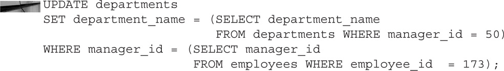
One subquery will run to determine the value of the department_name. The other subquery will run to determine which rows are to be changed.
DELETE
DELETE statements are simply used to remove a row from a table. Removing rows often seems anathema to many DBAs because data is their life. However, there may come a time when you need to remove rows from tables. In reality, Oracle does not actually delete the rows. It has a pointer that says that those data blocks can be used again. However, from the point of view of the users and the table, the data is permanently removed. It is not possible to delete values in just some columns. To perform such an action, you would use the UPDATE command.
In the following example, we are deleting a particular employee based on his employee number:

This next statement will delete all the rows matching department number 50:

In the following example, all the rows will be deleted because there is no WHERE clause:
![]()
NOTE
In certain instances, you will not be allowed to delete rows from a table. If there is a parent/child relationship, for example, you will be prevented from deleting the parent record because child records exist. A parent/child relationship is made via what is known as a foreign key constraint.
Not only could this be a bad thing to do, it can often be a very slow-running command if the table has millions and millions of rows. Deletes are typically an “expensive” performance operation in Oracle, and deleting millions of rows could affect performance.
If you want to delete all the rows in a table, you can use the TRUNCATE command. This command is a Data Definition Command (DDL) statement, and it is automatically committed. Because it is a DDL command, it cannot be rolled back, whereas a DELETE statement can be. We will talk about DDL commands and what COMMITs mean later in the chapter.
This final example shows that DELETE statements can also use subqueries to determine which rows to delete:

MERGE
Introduced in 9i, the MERGE statement is a really cool marriage of INSERT and UPDATE. In fact, it was originally called UPSERT. If the row does not exist, it is inserted into the table. If the row does exist, it is updated. MERGE also allows some more complex processing, including deletes and using subqueries.
In this example, we are putting data into the history_employees table:

Here, the column that is being matched, employee_id, is compared with the value in the employees table. If the values in the tables match, the manager_id in the history_employees table will be changed to 201. If they do not match, the rows would be inserted into the history_employees table. One thing to note here: we are using the letters h and e as table aliases. This allows us to not write out the whole table name but just to use the alias instead.
We can also put a SELECT statement into the USING clause rather than an actual table, as shown next:

Here, we are inserting rows into the history_employees table again. Rather than matching the employees table, rows will be a resulting data set to match from the subquery.
Transactions
We have skipped over a major important factor regarding DML statements: transactions. We should dive into the topic of transactions now that you have learned about DML statements. A transaction is simply a statement of work. A friend once called it “the stuff between commits.” When a change takes place in the database, it is not permanent until a “commit” happens. If you do not want to make it permanent, you can run what is known as a “rollback.” There are also these things known as savepoints, which you can think of as bookmarks. Only the users who have entered the DML statements are able to see the changes until they are committed. Other users, if querying the database, would see the old values.
NOTE
Oracle actually writes the value into the database block (in memory) and writes the before and after image into what is known as the redo buffer, which then gets written into an undo segment. The redo buffer then gets flushed out to the redo logs, where the before and after images can then be used for recovery purposes. If another user queries the table, they will actually be reading the undo segment rather than the data blocks. They will see the old values (from the undo segment) because the data has not been committed. Only the user who made the change will see the actual change until the data is committed.
COMMIT As mentioned, the DML statements are not permanent in the database until a commit happens. A commit tells the database to keep this data as the new “record.” A few things happen in the Oracle database (see the preceding Note), and the change is permanent. The command is one word:
![]()
Yes, it is a simple command that is executed. Let’s look at it in the context of a transaction:

The last commit shown would commit all DML statements up until the previous commit. This would then be the next commit point for future commits.
ROLLBACK The ROLLBACK command, shown next, is the opposite of the COMMIT command. It basically “erases” the transactions all the way to the last commit. All of the changes that the DML statements have made would be undone as if they never occurred and the previous state of the data is restored.
![]()
When you run this command, any previous changes made would not be put into the tables and the new “starting point” for the next transaction would be back to the last commit. Let’s look at this in terms of a transaction:
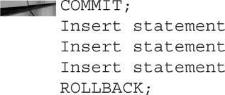
This ROLLBACK statement would “undo” all three “insert” statements. The previous commit would be the new “start” of the next transaction.
SAVEPOINT Savepoints can be considered bookmarks. You can place them anywhere within a transaction. At some point in the future, rather than rolling back to the start of the transaction, you can roll back to a savepoint. At that point in time, you can consider rolling back to the beginning of the transaction, rolling back to another savepoint (if it exists), or committing the transaction. You also have to name the savepoints, like so:
![]()
You can name them whatever you like, but giving them meaningful names will be much more helpful.
Let’s look at how you would use a savepoint with DML statements interspersed:

You now have at least four options. The next command could be
![]()
ROLLBACK;
![]()
ROLLBACK to POST_DELETE;
![]()
ROLLBACK to POST_INSERTS;
![]()
COMMIT;
You can now roll back, roll back to savepoint POST_DELETE, roll back to POST_INSERTS, or commit. One thing to note: if you roll back to savepoint POST_DELETE, there is no way to get those three inserts back—they are gone. Savepoints can be useful if you’re doing complex data manipulation. If you combine them with triggers and procedures (discussed further in this chapter), you can use logic to decide if you want to make the changes to the database permanent.
Data Definition Language
Data Definition Language (DDL) commands are not something you will use that often in regard to data integration, but we will look at a few here for the sake of completeness. DDL commands are used to create, modify, and drop objects. You don’t have to commit DDL commands. They have implicit commits. Conversely, you can’t roll them back.
If you have a few DML commands and then use a DDL command in the same session, that will commit the DML commands. Therefore, be very careful when running a DDL command while there are uncommitted transactions.

One DDL command that could be extremely useful to you in the world of data integration is Create Table As Select. This is often known by the abbreviation CTAS. Here is an example:
![]()
This will create a completely new table with the same structure and rows as the original employees table. You don’t have to have all the columns. You can just pick the columns you are interested in.
You can also put a WHERE clause in there to filter only certain rows, as shown here:

If you want to create a table with the same structure but without the actual rows, you can try the following command:

Using a WHERE clause that is false will create a table with the exact same structure as the original table, with the same columns you selected and column names; however, the table will contain no rows.
Data Control Language
Data Control Language (DCL), although an important part of SQL, is often used in conjunction with being a DBA; it’s not used much in regard to data integration. In some instances, developers and other users may be involved in granting permissions. Having the proper privileges is necessary to complete most of the other actions discussed in this chapter. For the sake of completeness, we will look at a bit of DCL.
DCL is used for the granting of privileges and the revoking of privileges. As seen in the following example, you can be very specific about what privileges you grant to certain users or roles. Conversely, you can also be specific about what privileges you revoke from the users.

SQL Summary
Using SQL is the most common way to retrieve data from a database—whether you are querying the database, manipulating the rows in the tables, changing the table structure, or granting permissions on those objects. By using combinations of different SQL statements you can control exactly what information you extract from the database. By combining this with the techniques you learn later in this chapter, you will have at your disposal ways to take the data and send it to other destinations.
As you have seen, SQL is a powerful language that allows you to query data from the database. You can grab large sets of data or get specific rows. DML statements allow you to add more data, modify the existing data, or remove the data from tables in the database. Also, the nature of transactions allows you to set boundaries for the particular changes as well as decide whether you want to make those changes permanent.
PL/SQL
As powerful as SQL is, there are some things that SQL just can’t do—and that’s why PL/SQL was created. Procedural Language/Structured Query Language was introduced in Oracle version 7. Unlike SQL, which is an ANSI standard and works on all RDBMS databases, PL/SQL only works on Oracle databases (although it has been recently ported to Oracle TimesTen and even IBM DB2 in later versions). PL/SQL is based on the programming language Ada, which was developed by the U.S. Department of Defense to replace the multitude of languages being used there. PL/SQL uses the basic models of syntax based on Ada. PL/SQL has some great advantages in that the code lives inside the database, which saves on compile time and is less expensive in terms of database overhead. PL/SQL can be used again and again by other users who have permission to use those objects. It is also reusable across versions and is typically enhanced as Oracle versions move forward.
NOTE
Ada was named after Ada Lovelace, the daughter of the English poet Lord Byron. Ada has often been called the world’s first programmer for her work with Charles Babbage’s mechanical general-purpose computer back in the 1800s.
PL/SQL allows users to create their own homemade functions versus just using the built-in functions that come with Oracle. It also has some things that SQL doesn’t have. PL/SQL allows the use of loops and condition operators, which adds quite a bit of functionality over SQL.
There are a few major different parts of PL/SQL. The basic code block is the anonymous block. The other parts of PL/SQL are made up of functions, procedures, packages, and triggers. These are often used to move, monitor, and track data changes, and all have their place in the data integration world. PL/SQL offers all the advantages of a procedural programming language, but lacks the performance of pure set-based SQL DML queries when being used for record-by-record manipulations.
Functions
A function is a standalone piece of code that returns a value. Oracle has dozens and dozens of built-in functions. These functions can be used right out of the box with regular SQL. However, there are many times when users might see the need to create customized functions to suit their business requirements, and for this reason PL/SQL functions have been created.
Use the following code to see all the Oracle built-in functions:

As with most objects in the Oracle databases, you will need to give the function a name. It should be unique and easy to use. Remember that the purpose of a function is to return a value to the user. You may want to name the function something related to what its purpose is. You will also want to ensure that the function returns one and only one value. An important thing to remember is that a function only has to have a unique name within a schema (a schema being defined as a collection of user objects). Here’s an example of a PL/SQL function:

This is a “simple” function. It is being created with the name sal_check, it has one input variable (called emp_id_var), and it will be a NUMBER data type. The output will be called salary_var and will also be a NUMBER data type. A SELECT statement will be run with the input variable used as the WHERE clause, and the output value is the result of that SELECT statement. The result is then given as the output value of the function.
Let’s look at an example of how to use the actual function:

User-made functions are used exactly how built-in Oracle functions are used. The body can have complex math or logic, but when the user calls the function, it returns a value. In this example, the function returns a simple value of the employee’s salary. (Note that in the SELECT statement there is no mention of the salary column.) The function could have added math or called on more complex operations. The SELECT statement is required to return exactly one value. If it had returned multiple values or no values at all, it would have returned an error. Dealing with multiple values or no values can be addressed inside the actual function.
Procedures
A stored procedure is simply a call to run a program saved in the database that contains one or more tasks. Like functions, procedures may have input parameters, but they are not necessarily required. However, unlike functions, procedures are not required to return a value, although they do have that option. Stored procedures can be used to perform business logic. Procedures can also be called from other packages, procedures, and triggers. Let’s take a look at a sample procedure:

To use the procedure, you can run it from the SQL*Plus prompt, as shown next. It can also be embedded in other places, such as other PL/SQL blocks, or it can be called from other programs running inside of Oracle.

NOTE
Although the variable followed by the => assignment operator is optional, it is good coding practice. It typically helps with readability and maintainability. It also helps avoid errors with misalignment of inserts.
Let’s look at what the procedure does. It has three input variables, and then performs a simple insert into a table. It takes the three input variables and places them into the correct columns. It also inserts into the employee column the value of a sequence. You can think of a sequence as a number generator. We also create an email by concatenating the last name with the email address, and we use the SYSDATE operator to automatically put in today’s date. There is also a commit call in the procedure to make the insert a permanent record in the database.
Procedures can be made quite large and complex, but to execute that code requires just a one-line command. The beauty here is that you can make a nice, simple call to the stored procedure and then the procedure goes off and does what it was programed to do. Procedures are a great way to make sure your business logic is stored in the database with repeatable code. This can be very powerful when combined with triggers, as you shall see shortly.
Packages
PL/SQL packages are simply groups of logically linked functions and procedures. It is very good practice to have your procedures as part of a package to allow for modularization of the code. Variables and subroutines can be shared and encapsulated within just that package. Here are a handful of reasons why you might want to put your procedures inside of a package:
![]() Unity The procedures and functions that are related can all be together in one place. This also makes for good change control because the functions and procedures are stored together and can be changed together.
Unity The procedures and functions that are related can all be together in one place. This also makes for good change control because the functions and procedures are stored together and can be changed together.
![]() Sharing The different variables and exceptions can be shared among the subroutines.
Sharing The different variables and exceptions can be shared among the subroutines.
![]() Safety You can have private procedures in a package that can’t be used elsewhere.
Safety You can have private procedures in a package that can’t be used elsewhere.
![]() Simple You only need to have one grant on a single package versus many procedures and functions.
Simple You only need to have one grant on a single package versus many procedures and functions.
The following is a simple package:

Here are some examples of how to use packages:

Packages can get quite complex, share variables and values, and have multiple functions and procedures. Only a snippet is shown here to introduce you to packages, because the topic of PL/SQL packages is quite a large one. Packages are not only logical groups, but they also build an own namespace for context, which is a very important aspect for variable definition and security.
Triggers
Triggers are often mentioned in talks about data integration. Indeed, before many of the real-time data integration tools such as Oracle GoldenGate and Dbvisit Replicate were developed, triggers were the main way to move data as “real time as possible.” Many of the early versions of replication tools were “trigger based,” especially before Oracle reformed their redo logs in Oracle 9.1. A trigger is a PL/SQL block that is to be fired when something occurs. Triggers have many different purposes. They can be used for a variety of reasons:
![]() Event logging
Event logging
![]() Auditing
Auditing
![]() Movement of data
Movement of data
![]() Changing data in tables
Changing data in tables
![]() Security
Security
One of the great features of triggers is that they can be enabled and disabled. This allows you to turn triggers off if you need to. Stored procedures have the ability to be invoked, but triggers do not. An “event” has to occur for a trigger to work. If the trigger is enabled and the event does occur, the trigger is fired. The four basic types of triggers are row triggers, statement triggers, “instead-of” triggers, and event triggers.
Row Triggers
Row triggers are extremely versatile. When you create the trigger, you can decide on exactly which DML operation you would like it to fire upon. This allows you to customize the trigger and focus on the exact business problem at hand. You can also determine whether you want the trigger to fire before or after the particular DML. By having it check before, you can determine whether you actually want the DML to go through. By having it check after, you can do some auditing or kick off some other background process. The key thing about a row trigger is that it will fire for each and every row that is affected by the particular DML. If the DML affects four rows, the trigger will fire each time. Consider the following example:

Here, you can see that we have two conditions. This trigger will fire before an insert or an update. There is also the clause FOR EACH ROW WHEN, which means that the trigger will fire for every row affected. In other words, if the insert or update changes several rows, the trigger will fire for each one of them. You will also notice a condition on this trigger as well. The result of the trigger is that a package with the name hr_salary containing the procedure commission_pay will fire.
Statement Triggers
Statement triggers are only fired one time. Even if the triggering event affects 200 rows, the trigger will only fire one time. In the following example, we have two triggers that will execute when an event occurs:

The first one will be after an insert is put into the employees table. The result will be a procedure, as part of a package, being fired. The second one is before a row is deleted, and it will fire off two different procedures. As opposed to the row-level triggers, these triggers will only fire one time.
Instead-of Triggers
Instead-of triggers do exactly what the name proclaims. They fire instead of the actual triggering statement. Instead-of triggers are row triggers, in that they will fire once for each row affected. These triggers are most often used to update views. Whereas simple views allow updates, complex views (such as those with aggregate functions, joins, and so on) do not allow updates. The instead-of triggers can be used to substitute DML on views. Consider the following example:

This trigger is created for when users try to insert into the employees_vu view. When an insert is performed against this view, the trigger will fire. As noted, it will do so once for each row. Rather than the row going into the view, the trigger will insert the new values into the employees table with a commit at the end.
Event Triggers
Event triggers come in two types: system events and user events. System trigger events are caused by database events such as the starting up or shutting down of an instance or server errors occurring on the database. A user event can be triggered by certain user activities such as performing DDL, DML, or logging off.
The following trigger is set to fire after every user logs on to the database. It takes the username along with the date (which also includes a timestamp) and inserts it into the logontab table, and then it commits.

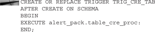
We can also set triggers to fire after a user creates schema objects. Here we have a procedure that will fire any time some user creates an object:
As mentioned previously, triggers can be turned on and off. There may be times when you are doing a bulk load of data and you don’t want the triggers firing. Or you may have an application or process for which you want to turn the trigger off for the time being. You can do this by altering the state of the trigger, as shown next:

And when you want to enable the trigger, it is also a simple command.
The COPY Command
The COPY command is not technically a SQL command but is part of the tool called SQL*Plus. It is probably not as well known as it should be. The COPY command has some great features that make it extremely useful. However, there is a caveat, from the official Oracle documentation:
“The COPY command is not being enhanced to handle datatypes or features introduced with, or after Oracle8i. The COPY command is likely to be made obsolete in a future release.”
The COPY command still works in Oracle 12c and customers still use it. Although it may not work in all scenarios for you, it is something to keep in your bag of tricks if you need to move data.
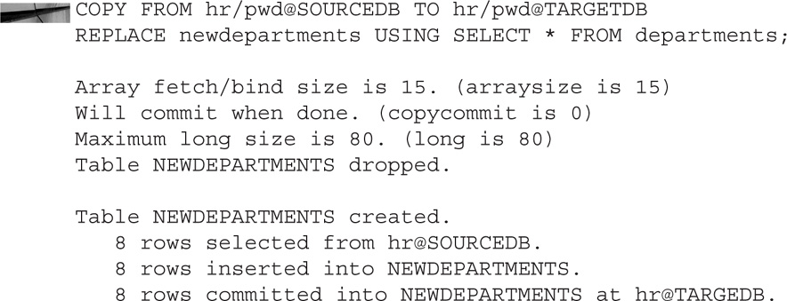
For example, suppose you would like to copy a table from one database to another:

This command will actually connect to the source database using the username and password provided, and then create and copy the table to the target database with the target username and password. The commit will occur at the very end. This is similar to Create Table As Select, except when using the COPY command we are going from one database to a completely different database.
If the table is already in existence, the previous command will fail. When the table already exists, use the REPLACE command instead, as shown here:
You can combine this with what you learned earlier and only pick certain columns, and you can use a WHERE clause to filter certain rows:

As mentioned before, the COPY command has been deprecated by Oracle and only supports certain data types:
![]() CHAR
CHAR
![]() DATE
DATE
![]() LONG
LONG
![]() NUMBER
NUMBER
![]() VARCHAR2
VARCHAR2
If you have tables that only contain those data types, feel free to make use of the COPY command.
SPOOL
By default, queries that are run are printed on the screen. Sometimes you want to have some of the dataset off the screen and in a flat file. The command in SQL*Plus to save the data in a file on the operating system is called SPOOL. This is a quick and easy way to get data from a query into a flat file on the operating system. This command is part of SQL*Plus and is not part of SQL. This is important to note because SPOOL is not an ANSI standard and therefore the code would not be portable.
Let’s look at how the SPOOL command is used. You enter the word SPOOL followed by the name of the file to which you would like the output written. The result set from your queries will still be presented to the screen, but anything you type in will also be piped to the named file. Here’s an example:

And now let’s look at the contents of the foo.txt file:

Combining the SPOOL command with a few other SQL*Plus commands can make the output very useful. We will turn off the headers for the columns as well as the feedback (the part that shows how many rows have been returned), and we will concatenate all the columns with a comma between each one:
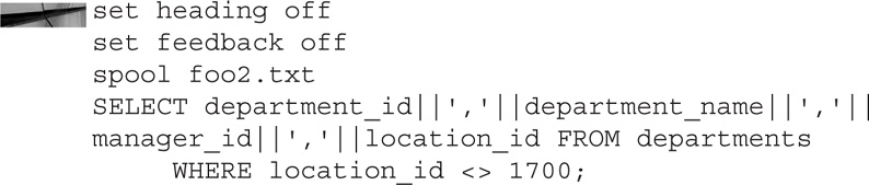
And here’s what we see when we look into the foo2 file:

As you can see, this is a nice output file with comma-separated values that can be used with other tools. Other querying tools such as SQL Developer and TOAD also have ways to spool out to a file. We’ve focused on the SQL*Plus SPOOL command here because just about all users of the Oracle database will has access to SQL*Plus.
SQL*Loader
Whereas SPOOL is a utility that takes data from the database and puts it into flat files, the utility SQL*Loader is used to take flat files on the operating system and put the data into tables inside the Oracle database. The SQL*Loader utility has been around for a long time. It has not had many enhancements, however, and does have some limitations. The “brains” of SQL*Loader is a file called the control file—not to be confused with the control file of the Oracle database. The control file contains the instructions on what SQL*Loader should do when started. You will also have a data file. The data file is simply that: a file that contains the data. Figure 2-1 shows the files used by SQL*Loader.

FIGURE 2-1. SQL*Loader files
Control File
The control file is the brains of SQL*Loader. It is well named because it truly does control the operations that will occur when SQL*Loader is invoked. The control file will tell SQL*Loader the following information:
![]() The name and location of the input data file
The name and location of the input data file
![]() What format the input data file has the records in
What format the input data file has the records in
![]() The name of the table or tables that will be loaded
The name of the table or tables that will be loaded
![]() The name and location of the discard file
The name and location of the discard file
![]() The name and location of the bad file
The name and location of the bad file
Let’s take a look at what’s inside a control file:
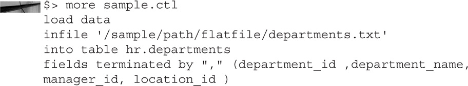
The first line, load data, tells SQL*Loader that data is to be loaded from a flat file on the operating system. The next line points to the location of the data file on the operating system. Next, we see which table will be loaded. The table must already exist and be empty. If the table already had rows in it, we can add the parameter APPEND before the keyword INTO. The last part of the control file mentions how the fields of the flat file are separated—in this case, they are separated by a comma—and then it lists what the fields are named.
Let’s look at invoking SQL*Loader using the control file:

Here is the data file, which is just data fields separated by commas:

Data fields don’t have to be separated by commas. You could of course use many different delimiters, although .csv (comma-separated values) files are the most common. It is even possible to use different delimiters in the same data file, like so:

Notice how the first two fields are separated by a comma and that an asterisk (*) and a percent sign (%) are used to separate the last three fields.
The control file would look like this:

In some cases, the data will not be separated by commas or any other character. You may get the data in what is known as fixed-length format, shown next. SQL*Loader can also deal with files in that format type.

In this case, the control file would just have to spell out exactly what fields are in what positions:

Sometimes the data might not be in exactly the format you want it. You can also manipulate the data as it passes through SQL*Loader from the data file:

This control file will do two things differently than the very first control file we looked at. The field department_id will have a one added to the value that is in the actual data file, and the value of department_name will have the built-in function initcap applied to it. This makes the first letter capital and the following letters lowercase. The remaining two fields will stay the same as in the data file.
There are also times when you might have a data file with millions of rows in it but you may only want certain rows inserted into the table in the database. Rather than performing that sorting in the flat file, you can use SQL*Loader to filter that data at run time:

The addition of the “when” clause is what allows the filter to work. Think of it as the WHERE clause in SQL you learned about earlier in this chapter. If the fields match the condition, they will be inserted into the table. If they do not match, they will be sent to what is known as the discard file, which we will discuss a bit later in the chapter.
This last example of a control file is a special one. If you are doing something one time and don’t need to use SQL*Loader multiple times, you can put the data file inside the control file. Instead of pointing to the location, you use an asterisk (*), and after the keyword begindata you can have the data just as you would in a “regular” data file. Here’s an example:

Dealing with the Bad File
So what happens if you are putting data into a table and the data is rejected? That is where the bad file comes into play. The bad file is aptly named. It is where bad records go if they are rejected by SQL*Loader or the database. They could be rejected by SQL*Loader for bad formatting or missing delimiters. Rows could be rejected by Oracle for not having required values, for having wrong data types in the wrong column, or for having keys that are not unique. A bad file is created automatically if one is not specified. It will have the same name as the data file but with the extension .bad. This makes it extremely useful because you can correct any mistakes and then just run that file through SQL*Loader a second time.
Whereas the bad file is created automatically, the discard file needs to be specified in the control file to be created. Rows that do not meet the criteria of the filter specified will be placed in the discard file. Even when you specify a discard file, it will only be created if there is occasion to, meaning that a discard file was specified in the control file and a record did not meet the criteria of the filter. Here’s an example:

Invoking SQL*Loader
You have three ways in which to invoke SQL*Loader. You can call SQL*Loader from the command line, in a parameter file, or interactively. You have seen that you can put all the commands on one line, like this:
![]()
You can also use SQL*Loader interactively. Type in sqlldr and the username, and the prompts will ask you for the control file and the password:

One of the most common methods of using SQL*Loader is through what is known as a parameter file, or par file for short. You place all the commands and parameters inside of a file and just have SQL*Loader call that one file, like so:
![]()
The inside of the testloader.txt file would look like this:

External Tables
External tables were introduced to Oracle in version 9i. External tables allow you to query data that is stored in flat files on the operating system versus having the data in the database. You can then treat the tables like you do other tables located in the database. You can query them, perform joins with them, and work with them as you would with a normal table. You cannot perform DMLs on these tables, though. The results from querying an external table are typically a bit slower than when querying a table that resides in the Oracle database. Figure 2-2 shows how an external table would look.

FIGURE 2-2. External table
We must first create a directory so that the database knows where to look for the table:
![]()
Now we will create the table itself. The first part of the create table statement looks similar to creating a table in the database. We then specify that the table is external and in the directory we named. We also mention how the records are stored in the flat file as well as the name of the flat file. Here’s an example:

Let’s look in the flat file before performing a query on the table:

And as shown here, you select against the table just like you would a regular table in the database. Users would have no idea that they are querying a flat file on the operating system.

Summary
With so many tools available, it can often be overwhelming to know which tools are the best. Learning SQL and all the different ways that SQL can be used is probably priority number one. Learning how transactions work is integral to learning how DML interacts with the Oracle database. As mentioned, DDL and DCL, although important, will not be as integral for use in data integration. PL/SQL can be extremely useful, but it really depends on exactly what you need. Triggers, when combined with packages and procedures, can really expand what you can do with the data. SQL*Loader has long been the go-to tool to get data that is stored in flat files into the Oracle database. SPOOL can help you get the data quickly from the database into a flat file. The use of external tables, although not necessarily very popular, can be useful if you have some outside tool populating the flat files and want to keep the data there. Finally, the COPY command of SQL*Plus, although deprecated, still has its place. Each of the tools mentioned in this chapter should be looked at individually and used as the occasion arises. Remember that practicing with each of these methods before you need them can make the going easier when it comes time to actually put them into use.