
11 Sets
Servile flattery—the kind made mostly of lies—will endear a lot of different kinds of people to you. Sycophancy wins friends and influences people. But I’ve never known anyone—and certainly none of the people I call “hero”—who chased after an elusive dream—one that required sacrifice, courage, resolve, or just plain mettle—and seized it through unctuous flattery. Edison, Jefferson, Lincoln, Einstein, Twain, Socrates, Confucius, Poe, Da Vinci, King—none of them fawned his way into history. Instead, they waged war against the toadies and trucklers of the world. They left indelible handprints on the past because they had the audacity to be honest and because they knew the difference between loyalty and servility.—Trace Ambraise
Given that the relational model is based on sets of tuples, it should come as no surprise that SQL Server provides a rich suite of tools for working with sets of rows. The set is the focal point of work in SQL Server—the server resolves the queries you pass it by returning sets—result sets. It stores sets of rows together in tables (or bags) and relates sets to one another via Declarative Referential Integrity and joins. That it provides such comprehensive set support is to be expected—sets are the life’s blood of relational databases.
The ANSI SQL-92 set operation keywords—UNION, EXCEPT, and INTERCEPT—are used to determine set union, difference, and intersection, respectively (sets are assumed to be collections of rows). Though Transact-SQL supports only one of these directly—UNION—it’s straightforward to perform the other operations using simple coding techniques. SQL is a set-oriented language; working with sets of records is what it does best.
Performing a set union is trivial in Transact-SQL thanks to the inclusion of the UNION keyword. Here’s some sample code that combines two sets using the UNION operator:

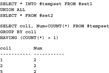
Note that the column names of the two tables differ in this example. All that’s required of SELECT statements joined via UNION is that they have the same number of columns and that each column’s data type either matches its counterpart or is capable of being implicitly converted to it. The SELECT statements themselves can be as complex as necessary, though they may not include COMPUTE, ORDER BY, or FOR BROWSE. You can use COMPUTE and ORDER BY with the result set returned by the UNION operation but not with any of its individual SELECT statements. Conversely, GROUP BY and HAVING can be used by individual SELECT statements but not by the entire result set. This is a pretty serious limitation, but fortunately there’s a workaround. Here’s some code that shows a way of using GROUP BY and HAVING with result sets created by UNION:

This approach uses a derived table to wrap the UNION result set, then groups and qualifies it using GROUP BY and HAVING. An alternative would be to encapsulate the UNION operation in a view, but the illustrated approach is more expedient since it doesn’t involve the creation of a separate object.
Note the use of UNION ALL in the example code. Normally, UNION removes duplicates from its result set by sorting or hashing them. Obviously, this can take time. If you know your result set is already free of duplicates or if you don’t care whether it contains duplicates, UNION ALL can be a much faster way of combining tables. It simply combines the results of its component SELECTs and returns them—there’s no sorting or duplicate elimination. It’s needed by the query above because we want to apply a HAVING clause that filters the result set according to the number of instances of each col1 value. Obviously, we can’t do that if UNION removes all duplicates, effectively restricting the number of instances of each value to just one. So, we use UNION ALL within the derived table, then remove duplicates and aggregate our results using the GROUP BY of the outer SELECT.

Caution
Avoid mixing UNION and UNION ALL if you can. If duplicates are removed in some cases but not in others, you may end up with a result set that is difficult to interpret. The individual SELECT statements composing a compound UNION operation cease to be associative when UNION and UNION ALL are mixed. This means, by extension, that Transact-SQL’s left-to-right order of execution will affect the result set.
Transact-SQL provides a nifty enhancement to SQL’s standard UNION syntax that allows a table to be created en passant. To do this, you include an INTO tablename clause in the first SELECT statement of those included in the UNION operation, like so:
This code first creates a table via the UNION construct, then queries it via a separate SELECT statement. This technique is better than the derived table approach if you need to process the UNION result set further following the operation.
ANSI SQL-92 defines the EXCEPT keyword for returning a result set consisting of the difference between two sets. Most SQL vendors, including Microsoft, have yet to implement this keyword (Oracle has the MINUS synonym), but since Transact-SQL is a set-oriented language at heart, determining the difference between two sets isn’t a difficult task.
The most obvious way to determine the rows that exist in one set but not in another is via the EXISTS predicate. Here’s a code sample that returns the rows in one table that do not exist in another:

This method uses a correlated subquery to find the rows in #set1 that do not exist in #set2. Note that this method requires each column in each table to be matched up individually. This can quickly become very cumbersome when dealing with tables with lots of columns.
Unlike the ANSI SQL EXCEPT construct, this solution returns duplicate rows if they exist in the first table. To remedy this, insert the DISTINCT keyword in the outer SELECT.
A more efficient way to return the difference between two sets is to use a simple OUTER join. This alleviates the need for a correlated subquery, so it’s not only faster but also easier to read:

The approach works by virtue of the fact that a left outer join returns columns from the rightmost table as NULL when the join condition fails. The query simply limits the rows it returns to those where this occurs. In other words, it restricts the rows returned from the leftmost table to those that don’t exist in the right-side table. As in the previous example, this technique requires that every column in the first set be compared with its counterpart in the second set, which gets tedious with lots of columns.
One type of set that neither of these approaches handles very well is one containing duplicates. Codd’s relational model and basic set theory prohibit duplicate set elements, but ANSI/ ISO SQL permits them and so does Transact-SQL. That’s why tables are sometimes referred to as “multisets”—they may contain multiple sets that individually contain unique elements.
The issues that arise when duplicates are present in a set are many and varied. If the first set contains two instances of a given row, but the second contains just one, what should we do? A result set that shows the difference between the two sets should include from the first set duplicate rows that have no matches in the second set. It shouldn’t exclude the row from the result set simply because there’s a match for an earlier duplicate in the second set.
Unfortunately, neither of the techniques presented thus far can handle this situation. Regardless of how many times a given row appears in the first set, if it occurs even once in the second set, it’s not included in the difference set. Here’s a query that ensures that each set has at least as many copies of a given row as the other set before a match is assumed (I’ve altered the sets to include duplicate rows):
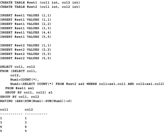
Even though row (1,1) appears in both sets, this query returns the row in the difference set because it appears more times in the first set than in the second. Similarly, even though (5,5) appears in both sets, it appears more times in the second set than in the first, so it’s included in the result set.
As with set differences, returning simple set intersections is easy using the EXISTS predicate. Here’s an example:
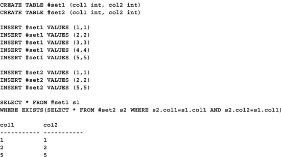
Like the initial set difference query, this one requires that each field in the first set be compared with its counterpart in the second. Each row in the first set whose columns match those of the second is then returned by the query. The result is the intersection of the two sets—those rows contained in both sets.
A more efficient way to return the intersection of two sets is simply to join them. An inner join works nicely for this since it omits rows without matches. Here’s an example:

It’s syntactically more compact and faster and is the most common way that set intersections are returned in SQL.
As with the set difference techniques, both of these techniques are unable to handle duplicates correctly. A single row in the second set may match up to two or more rows in the first set—there’s no provision for ensuring that a row appears the same number of times in each set before a match is assumed. Here’s a query that addresses this:
CREATE TABLE #set1 (col1 int, col2 int)
CREATE TABLE #set2 (col1 int, col2 int)
INSERT #set1 VALUES (1,1)
INSERT #set1 VALUES (1,1)
INSERT #set1 VALUES (2,2)
INSERT #set1 VALUES (3,3)
INSERT #set1 VALUES (4,4)
INSERT #set1 VALUES (5,5)
INSERT #set2 VALUES (1,1)
INSERT #set2 VALUES (2,2)
INSERT #set2 VALUES (2,2)
INSERT #set2 VALUES (4,4)
INSERT #set2 VALUES (5,5)
SELECT col1, col2
FROM (SELECT col1,
col2,
Num1=COUNT(*),
Num2=(SELECT COUNT(*) FROM #set2 ss2 WHERE col1=ss1.col1 AND col2=ss1.col2)
FROM #set1 ss1
GROUP BY col1, col2) s1
GROUP BY col1, col2
HAVING SUM(Num1)=SUM(Num2)

This approach uses a derived table and a subquery to count the number of rows that appear in each set for each pair of values. It then restricts the rows it returns to those that appear the same number of times in each set. In this case, (1,1) is excluded because it appears twice in the first set but only once in the second. Likewise, (2,2) is excluded because it appears twice in the second set but only once in the first.
Determining set intersection based on the number of times a row appears may amount to nothing more than an academic exercise in many cases. You may not care that the counts are different—you may want to know only when the two sets share a common value. If that’s the case, the first two techniques presented will accomplish the task with a minimum of code.
Of course, the easiest way to locate a portion of a set—a subset—is with a SELECT statement and a WHERE clause. That’s the most direct route and the one most often traveled.
Beyond that, though, what if you need something that, at least on the surface, appears to be too difficult for the WHERE clause? Take the problem of returning the top n rows in a set. What’s the best way to do this?
There are a number of approaches to this problem. Some of them are presented elsewhere in this book (e.g., see the section “Returning” the Top n Rows" in Chapter 8), so I won’t bother going into them here. Though it’s also covered adequately elsewhere in the book, the TOP n extension to the SELECT command is worth mentioning here in the context of sets and subsets. By far the most straightforward way to return the top portion of a set is via the TOP n clause, like this:

SET ROWCOUNT also works nicely for this, though, at least for SELECTs, TOP n is preferable because it doesn’t require a separate SQL statement. Here’s a version of the previous query that uses SET ROWCOUNT:
SET ROWCOUNT 3
SELECT State, Region, Population
FROM #1996_POP_ESTIMATE
ORDER BY Population DESC
SET ROWCOUNT 0 -- Reset ROWCOUNT
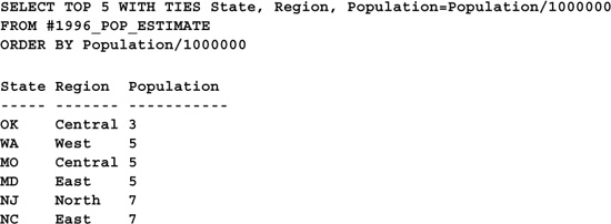
One distinct advantage the TOP n approach has over SET ROWCOUNT is in its ability to handle ties. The WITH TIES clause allows TOP n to include ties in the result set when an ORDER BY clause is used. Consider this variation on the earlier query:

It lists the top five states in population based on millions of people. Only whole millions are considered—fractional parts are truncated. Without the TIES option, the query can’t recognize the fact that there’s actually a tie for fifth place. New Jersey and North Carolina each had a population in excess of 7 million people in 1996. Here’s the query with the TIES option in place, along with its result set:

Because ORDER BY supports both ascending and descending sorts, TOP n can be used to retrieve the bottommost rows from a set as well, like so:
If you wish to order the result set returned by TOP n differently (let’s say you’d like the result set above in descending order, for example), you can easily embed it within a derived table and sort it using a separate ORDER BY clause, like so:

Beyond lopping off the rows at the extremities of a set, you may wish to extract them based on position. For example, you may wish to pull the odd- or even-numbered items from a set or, perhaps, every third item or every fifth and so on. This is the same basic problem as returning an interval from a sequence or run. The examples in Chapter 9, “Runs and Sequences,” illustrate how to return intervals that are larger than one row in size and that can have other complex criteria attached to them. For the time being, here’s a query that illustrates how to return all the even-numbered items in a set:
CREATE TABLE #set1 (k1 int identity)
INSERT #set1 DEFAULT VALUES
INSERT #set1 DEFAULT VALUES
INSERT #set1 DEFAULT VALUES
INSERT #set1 DEFAULT VALUES
INSERT #set1 DEFAULT VALUES
INSERT #set1 DEFAULT VALUES
INSERT #set1 DEFAULT VALUES
INSERT #set1 DEFAULT VALUES
INSERT #set1 DEFAULT VALUES
INSERT #set1 DEFAULT VALUES
SELECT s1.k1
FROM #set1 s1 JOIN #set1 s2 ON (s1.k1 >= s2.k1)
GROUP BY s1.k1
HAVING (COUNT(*) % 2) = 0
k1
-----------
2
4
6
8
10
This approach uses the familiar self-JOIN/GROUP BY technique, introduced earlier in this book, to compare the table with itself. It then uses the modulus operator (%) to restrict the rows it returns to even-numbered ones. Of course, you could change the =0 to =1 in order to return the odd-numbered rows, like so:
SELECT s1.k1
FROM #set1 s1 JOIN #set1 s2 ON (s1.k1 >= s2.k1)
GROUP BY s1.k1
HAVING (COUNT(*) % 2) = 1
k1
-----------
1
3
5
7
9
Transact-SQL is a set-oriented language. This is one of its strengths as a query tool and one of the chief advantages it holds over traditional programming languages. It was designed from the start to work with data in sets. Even though only one set-oriented operator is supported directly by Transact-SQL, finding the union, difference, or intersection between two sets is trivial compared to 3GL-based solutions. The relational model on which SQL Server is based makes these kinds of tasks quite straightforward.