
8 Statistical Functions
Statistics are like a bikini. What they reveal is suggestive, but what they conceal is vital.—Aaron Levenstein
There’s a common misconception by many developers—advanced and beginner alike—that SQL Server is unsuitable for performing complex computations. The perception is that it’s really just a data retrieval facility—it’s superb at storing and querying data, but any heavy calculation work must be performed in a 3GL of some sort. Though data management and retrieval are certainly its strong suit, SQL Server can perform complex calculations as well, including statistical calculations. If you know what you’re doing, there are very few statistical computations beyond the reach of basic Transact-SQL.
Capabilities notwithstanding, on the surface, SQL Server may seem like an odd tool to use to compute complex statistical numbers. Just because a tool is capable of performing a task doesn’t mean that it’s the best choice for doing so. After all, SQL Server is a database server, right? It’s an inferior choice for performing high-level mathematical operations and complex expression evaluation, right? Wrong. Transact-SQL’s built-in support for statistical functions together with its orientation toward sets makes it quite adept at performing statistical computations over data stored in SQL Server databases. These two things—statistical functions and set orientation—give Transact-SQL an edge over many 3GL programming languages. Statistics need data, so what better place to extrapolate statistics from raw data than from the server storing it? If the supermarket has all the items you need at the right price, why drive all over town to get them?
Notice that I didn’t mention anything about calling external functions written in traditional programming languages such as C++. You shouldn’t have to resort to external functions to calculate most statistics. What Transact-SQL lacks as a programming language, it compensates for as a data language. Its orientation toward sets and its ease of working with them yield a surprising amount of computational power with a minimum of effort, as the examples later in the chapter illustrate.
Another item I’ve left out of the discussion is the use of stored procedures to perform complex calculations. If you ask most SQL developers how to calculate the statistical median of a column in a SQL Server table, they’ll tell you that you need a stored procedure. This procedure would likely open a cursor of some sort to locate the column’s middle value. While this would certainly work, it isn’t necessary. As this chapter will show, you don’t need stored procedures to compute most statistical values, normal SELECTs will do just fine. Iterating through tables using traditional looping techniques is an “un-SQL” approach to problem solving and is something you should avoid when possible (See Chapter 13, “Cursors,” for more information). Use Transact-SQL’s strengths to make your life easier, don’t try to make it something it isn’t. Attempting to make Transact-SQL behave like a 3GL is a mistake—it’s not a 3GL. Doing this would be just as dubious and fraught with difficulty as trying to make a 3GL behave like a data language. Forcing one type of tool to behave like another is like forcing the proverbial square peg into a round hole—it probably won’t work and will probably lead to little more than an acute case of frustration.
One thing to keep in mind when performing complex mathematical calculations with Transact-SQL is that SQL, as a language, does not handle floating point rounding errors. Naturally, this affects the numbers produced by queries. It can make the same query return different results based solely on the order of the data. The answer is to use fixed point types such as decimal and numeric rather than floating point types such as float and real. See the section “Floating Point Fun” in Chapter 2 for more information.
Its clunky language syntax notwithstanding, CASE is an extremely powerful weapon in the Transact-SQL arsenal. It allows us to perform complex calculations during SELECT statements that previously were the exclusive domain of arcane functions and stored procedures. Some of these solutions rely on a somewhat esoteric technique of coding Transact-SQL expressions such that the number of passes through a table is greatly reduced. This, in turn, yields better performance and code that is usually more compact than traditional coding techniques. This is best explained by way of example. Let’s look at a function-based solution that creates a cross-tabulation or “pivot” table.
Assuming we have this table and data to begin with:
CREATE TABLE #YEARLY_SALES
(SalesYear smalldatetime,
Sales money)
INSERT #YEARLY_SALES VALUES ('19990101',86753.09)
INSERT #YEARLY_SALES VALUES ('20000101',34231.12)
INSERT #YEARLY_SALES VALUES ('20010101',67983.56)
here’s what a function-based pivot query would look like:
SELECT
"1999"=SUM(Sales*(1-ABS(SIGN(YEAR(SalesYear)-1999)))),
"2000"=SUM(Sales*(1-ABS(SIGN(YEAR(SalesYear)-2000)))),
"2001"=SUM(Sales*(1-ABS(SIGN(YEAR(SalesYear)-2001))))
FROM #YEARLY_SALES
1999 2000 2001
--------------------- --------------------- ---------------------
86753.0900 34231.1200 67983.5600
Note the inclusion of the rarely used ABS() and SIGN() functions. This is typical of function-based solutions and is what makes them so abstruse. The term “characteristic function” was first developed by David Rozenshtein, Anatoly Abramovich, and Eugene Birger in a series of articles for the SQL Forum publication several years ago to describe such solutions. The characteristic function above is considered a “point characteristic function” for the SalesYear column. Each instance of it returns a one when the year portion of SalesYear equals the desired year and a zero otherwise. This one or zero is then multiplied by the Sales value in each row to produce either the sales figure for that year or zero. The end result is that each column includes just the sales number for the year mentioned in the expression—exactly what we want.
Understanding how a characteristic function works within the context of a particular query requires mentally translating characteristic formulae to their logical equivalents. When characteristic functions were first “discovered,” tables were published to help SQL developers through the onerous task of doing this. This translation is necessary because the problems being solved rarely lend themselves intuitively to the solutions being used. That is, pivoting a table has nothing to do with the ABS() and SIGN() functions. This is where CASE comes in.
With the advent of SQL-92 and CASE, the need for odd expressions like these to build complex inline logic has all but vanished. Instead, you should use CASE whenever possible in place of characteristic functions. CASE is easier to read, is easier to extend, and requires no mental translation to and from arcane expression tables. For example, here’s the pivot query rewritten to use CASE:
SELECT
"1999"=SUM(CASE WHEN YEAR(SalesYear)=1999 THEN Sales ELSE NULL END),
"2000"=SUM(CASE WHEN YEAR(SalesYear)=2000 THEN Sales ELSE NULL END),
"2001"=SUM(CASE WHEN YEAR(SalesYear)=2001 THEN Sales ELSE NULL END)
FROM #YEARLY_SALES
1999 2000 2001
--------------------- --------------------- ---------------------
86753.0900 34231.1200 67983.5600
It’s vastly clearer and easier to understand than the earlier method involving SIGN() and ABS(). I also find it easier to read than:
SELECT
"1999"=SUM(CASE YEAR(SalesYear) WHEN 1999 THEN Sales ELSE NULL END),
"2000"=SUM(CASE YEAR(SalesYear) WHEN 2000 THEN Sales ELSE NULL END),
"2001"=SUM(CASE YEAR(SalesYear) WHEN 2001 THEN Sales ELSE NULL END)
FROM #YEARLY_SALES
Though this solution still represents a vast improvement over the SIGN()/ABS() approach, I prefer the searched CASE approach simply because the relationship between “1999” and YEAR(SalesYear) is more explicit in the searched CASE syntax, though I’d concede that this is really a matter of preference.
You’ll notice the liberal use of self-joins in the examples in this chapter. Techniques that involve self-joins over large tables should be viewed with a certain amount of skepticism because they can lead to serious runtime performance problems. This is also true of queries that make use of Cartesian products or cross-joins. I mention this only to forewarn you to be on the lookout for techniques that may be syntactically compact but extremely inefficient in terms of runtime performance. The key to successful SQL development is to strike a balance between the two.
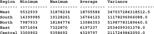
Transact-SQL sports nine different aggregate functions, all of which are useful for computing statistics. Beyond the “standard” aggregate functions you see in most SQL DBMS products—SUM(), MIN(), MAX(), COUNT(), and AVG()—SQL Server provides four that are specifically related to financial and statistical calculations: STDDEV(), STDDEVP(), VAR(), VARP(). The STDDEV functions compute sample standard deviation and population standard deviation, respectively, while the VAR functions compute sample variance and population variance. These functions work just like the other aggregate functions—they ignore NULLs, can be used with GROUP BY to create vector aggregates, and so forth. Here’s an example that uses Transact-SQL’s built-in aggregate functions to compute some basic statistics:
CREATE TABLE #1996_POP_ESTIMATE (Region char(7), State char(2), Population int)
INSERT #1996_POP_ESTIMATE VALUES ('West', 'CA',31878234)
INSERT #1996_POP_ESTIMATE VALUES (’South', ’TX',19128261)
INSERT #1996_POP_ESTIMATE VALUES ('North', 'NY',18184774)
INSERT #1996_POP_ESTIMATE VALUES (’South', 'FL',14399985)
INSERT #1996_POP_ESTIMATE VALUES ('North', 'NJ', 7987933)
INSERT #1996_POP_ESTIMATE VALUES ('East', 'NC', 7322870)
INSERT #1996_POP_ESTIMATE VALUES ('West', 'WA', 5532939)
INSERT #1996_POP_ESTIMATE VALUES ('Central','MO', 5358692)
INSERT #1996_POP_ESTIMATE VALUES ('East', 'MD', 5071604)
INSERT #1996_POP_ESTIMATE VALUES ('Central','OK', 3300902)
SELECT Region, MIN(Population) AS Minimum, MAX(Population)
AS Maximum, AVG(Population) AS Average, VAR(Population) AS
Variance, VARP(Population) AS VarianceP, STDEV(Population) AS
StandardDeviation, STDEVP(Population) AS StandardDeviationP
FROM #1996_POP_ESTIMATE
GROUP BY Region
ORDER BY Maximum DESC
(Results abridged)
Row-positioning problems—i.e., locating rows based on their physical position within a distribution—have historically been a bit of challenge in SQL. Locating a row by value is easy with a set-oriented language; locating one based on position is another matter. Medians are row-positioning problems. If there is an odd number of values in the distribution, the median value is the middle value, above and below which exist equal numbers of items. If there is an even number of values, the median is either the average of the two middle values (for financial medians) or the lesser of them (for statistical medians).
Row-positioning problems are greatly simplified when a unique, sequential integer key has been established for a table. When this is the case, the key becomes a virtual record number, allowing ready access to any row position in the table similarly to an array. This can allow medians to be computed almost instantly, even over distribution sets with millions of values. Here’s an example:
SET NOCOUNT ON
USE GG_TS
IF (OBJECT_ID('financial_median') IS NOT NULL)
DROP TABLE financial_median
GO
DECLARE @starttime datetime
SET @starttime=GETDATE()
CREATE TABLE financial_median
(
c1 float DEFAULT (
(CASE (CAST(RAND()+.5 AS int)*-1) WHEN 0 THEN 1 ELSE -1 END)*(CAST(RAND() *
100000 AS int) % 10000)*RAND()),
c2 int DEFAULT 0
)
-- Seed the table with 10 rows
INSERT financial_median DEFAULT VALUES
INSERT financial_median DEFAULT VALUES
INSERT financial_median DEFAULT VALUES
INSERT financial_median DEFAULT VALUES
INSERT financial_median DEFAULT VALUES
INSERT financial_median DEFAULT VALUES
INSERT financial_median DEFAULT VALUES
INSERT financial_median DEFAULT VALUES
INSERT financial_median DEFAULT VALUES
INSERT financial_median DEFAULT VALUES
-- Create a distribution of a million values
WHILE (SELECT TOP 1 rows FROM sysindexes WHERE id=OBJECT_ID('financial_median')
ORDER BY indid)< 1000000 BEGIN
INSERT financial_median (c2) SELECT TOP 344640 c2 FROM financial_median
END
SELECT 'It took '+CAST(DATEDIFF(ss,@starttime,GETDATE()) AS varchar)+' seconds
to create and populate the table'
SET @starttime=GETDATE()
-- Sort the distribution
CREATE CLUSTERED INDEX c1 ON financial_median (c1)
ALTER TABLE financial_median ADD k1 int identity
DROP INDEX financial_median.c1
CREATE CLUSTERED INDEX k1 ON financial_median (k1)
SELECT 'It took '+CAST(DATEDIFF(ss,@starttime,GETDATE()) AS varchar)+' seconds
to sort the table'
GO
-- Compute the financial median
DECLARE @starttime datetime, @rows int
SET @starttime=GETDATE()
SET STATISTICS TIME ON
SELECT TOP 1 @rows=rows FROM sysindexes WHERE id=OBJECT_ID('financial_median')
ORDER BY indid
SELECT ’There are '+CAST(@rows AS varchar)+' rows'
SELECT AVG(c1) AS "The financial median is" FROM financial_median
WHERE k1 BETWEEN @rows / 2 AND (@rows / 2)+SIGN(@rows+1 % 2)
SET STATISTICS TIME OFF
SELECT 'It took '+CAST(DATEDIFF(ms,@starttime,GETDATE()) AS varchar)+' ms to compute the financial median'
--------------------------------------------------------------------------------
It took 73 seconds to create and populate the table
The clustered index has been dropped.
--------------------------------------------------------------
It took 148 seconds to sort the table
--------------------------------------------
There are 1000000 rows
The financial median is
----------------------------------------------------
-1596.1257544255732
SQL Server Execution Times:
CPU time = 0 ms, elapsed time = 287 ms.
-----------------------------------------------------------------------
It took 290 ms to compute the financial median
This query does several interesting things. It begins by constructing a table to hold the distribution and adding a million rows to it. Each iteration of the loop fills the c1 column with a new random number (all the rows inserted by a single operation get the same random number). The table effectively doubles in size with each pass through the loop. The top 344,640 rows are taken with each iteration in order to ensure that the set doesn’t exceed a million values. The 344,640 limitation isn’t significant until the final pass through the loop—until then it grabs every row in financial_median and reinserts it back into the table (after the next-to-last iteration of the loop, the table contains 655,360 rows; 344,640 = 1,000,000-655,360). Though this doesn’t produce a random number in every row, it minimizes the time necessary to build the distribution so we can get to the real work of calculating its median.
Next, the query creates a clustered index on the table’s c1 column in order to sort the values in the distribution (a required step in computing its median). It then adds an identity column to the table and switches the table’s clustered index to reference it. Since the values are already sequenced when the identity column is added, they end up being numbered sequentially by it.
The final step is where the median is actually computed. The query looks up the total number of rows (so that it can determine the middle value) and returns the average of the two middle values if there’s an even number of distribution values or the middle value if there’s an odd number.
In a real-world scenario, it’s likely that only the last step would be required to calculate the median. The distribution would already exist and be sorted using a clustered index in a typical production setup. Since the number of values in the distribution might not be known in advance, I’ve included a step that looks up the number of rows in the table using a small query on sysindexes. This is just for completeness—the row count is already known in this case because we’re building the distribution and determining the median in the same query. You could just as easily use a MAX(k1) query to compute the number of values since you can safely assume that the k1 identity column is seeded at one and has been incremented sequentially throughout the table. Here’s an example:
DECLARE @starttime datetime, @rows int
SET @starttime=GETDATE()
SET STATISTICS TIME ON
SELECT @rows=MAX(k1) FROM financial_median
SELECT ’There are '+CAST(@rows AS varchar)+' rows'
SELECT AVG(c1) AS "The financial median is" FROM financial_median
WHERE k1 BETWEEN @rows / 2 AND (@rows / 2)+SIGN(@rows+1 % 2)
SET STATISTICS TIME OFF
SELECT 'It took '+CAST(DATEDIFF(ms,@starttime,GETDATE()) AS varchar)+' ms to compute the financial median'
Note the use of the SIGN() function in the median computation to facilitate handling an even or odd number of values using a single BETWEEN clause. The idea here is to add 1 to the index of the middle value for an even number of values and 0 for an odd number. This means that an even number of values will cause the average of the two middle values to be taken, while an odd number will cause the average of the lone middle value to be taken—the value itself. This approach allows us to use the same code for even and odd numbers of values.
Specifically, here’s how this works: the SIGN() expression adds one to the number of values in the distribution set in order to switch it from odd to even or vice versa, then computes the modulus of this number and 2 (to determine whether we have an even or odd number) and returns either 1 or 0, based on its sign. So, for 1,000,000 rows, we add 1, giving us 1,000,001, then take the modulus of 2, which is 1. Next, we take the SIGN() of the number, which is 1, and add it to the number of rows (divided by 2) in order to compute the k1 value of the second middle row. This allows us to compute the AVG() of these two values in order to return the financial median. For an odd number of values, the modulus ends up being 0, resulting in a SIGN() of 0, so that both terms of the BETWEEN clause refer to the same value—the set’s middle value.
The net effect of all this is that the median is computed almost instantaneously. Once the table is set up properly, the median takes less than a second to compute on the relatively scrawny 166 MHz laptop on which I'm writing this book. Considering that we’re dealing with a distribution of a million rows, that’s no small feat.
This is a classic example of SQL Server being able to outperform a traditional programming language because of its native access to the data. For a 3GL to compute the median value of a 1,000,000-value distribution, it would probably load the items into an array from disk and sort them. Once it had sorted the list, it could retrieve the middle one(s). This last process—that of indexing into the array—is usually quite fast. It’s the loading of the data into the array in the first place that takes so long, and it’s this step that SQL Server doesn’t have to worry about since it can access the data natively. Moreover, if the 3GL approach loads more items than will fit in memory, some of them will be swapped to disk (virtual memory), obviously slowing down the population process and the computation of the median.
For example, consider this scenario: A 3GL function needs to compute the financial median of a distribution set. It begins by loading the entire set from a SQL Server database into an array or linked list and sorting it. Once the array is loaded and sorted, the function knows how many rows it has and indexes into or scans for the middle one(s). Foolishly, it treats the database like a flat file system. It ignores the fact that it could ask SQL Server to sort the items before returning them. It also ignores the fact that it could query the server for the number of rows before retrieving all of them, thus alleviating the need to load the entire distribution into memory just to count the number of values it contains and compute its median. These two optimizations alone—allowing the server to sort the data and asking it for the number of items in advance—are capable of reducing the memory requirements and the time needed to fill the array or list by at least half.
But SQL Server itself can do even better than this. Since the distribution is stored in a database with which the server can work directly, it doesn’t need to load anything into an array or similar structure. This alone means that it could be orders of magnitude faster than the traditional 3GL approach. Since the data’s already “loaded,” all SQL Server has to concern itself with is locating the median value, and, as I’ve pointed out, having a sequential row identifier makes this a simple task.
To understand why the Transact-SQL approach is faster and better than the typical 3GL approach, think of SQL Server’s storage mechanisms (B-trees, pages, extents, etc.) as a linked list—a very, very smart linked list—a linked list that’s capable of keeping track of its total number of items automatically, one that tracks the distribution of values within it, and one that continuously maintains a number of high-speed access paths to its values. It’s a list that moves itself in and out of physical memory via a very sophisticated caching facility that constantly balances its distribution of values and that’s always synchronized with a permanent disk version so there’s never a reason to load or store it explicitly. It’s a list that can be shared by multiple users and to which access is streamlined automatically by a built-in query optimizer. It’s a list than can be transparently queried by multiple threads and processors simultaneously—that, by design, takes advantage of multiple Win32 operating system threads and multiple processors.
From a conceptual standpoint, SQL Server’s storage/retrieval mechanisms and a large virtual memory–based 3GL array or linked list are not that different; it’s just that SQL Server’s facilities are a couple orders of magnitude more sophisticated and refined than the typical 3GL construct. Not all storage/retrieval mechanisms are created equal. SQL Server has been tuned, retuned, worked, and reworked for over ten years now. It’s had plenty of time to grow up—to mature. It’s benefited from fierce worldwide competition on a number of fronts throughout its entire life cycle. It has some of the best programmers in the world working year-round to enhance and speed it up. Thus it provides better data storage and retrieval facilities than 95% of the 3GL developers out there could ever build. It makes no sense to build an inferior, hackneyed version of something you get free in the SQL Server box while steadfastly and inexplicably using only a small portion of the product itself.
One thing we might consider is what to do if the distribution changes fairly often. What happens if new rows are added to it hourly, for example? The k1 identity column will cease to identify distribution values sequentially, so how could we compute the median using the identity column technique? The solution would be to drop the clustered index on k1 followed by the column itself and repeat the sort portion of the earlier query, like so:
DROP INDEX financial_median.k1
ALTER TABLE financial_median DROP COLUMN k1
CREATE CLUSTERED INDEX c1 ON financial_median (c1)
ALTER TABLE financial_median ADD k1 int identity
DROP INDEX financial_median.c1
CREATE CLUSTERED INDEX k1 ON financial_median (k1)
Obviously, this technique is impractical for large distributions that are volatile in nature. Each time the distribution is updated, it must be resorted. Large distributions updated more than, say, once a day are simply too much trouble for this approach. Instead, you should use one of the other median techniques listed below.
Note that it’s actually faster overall to omit the last two steps in the sorting phase. If the clustered index on c1 is left in place, computing the median takes noticeably longer (1–2 seconds on the aforementioned laptop), but the overall process of populating, sorting, and querying the set is reduced by about 15%. I’ve included the steps because the most common production scenario would have the data loaded and sorted on a fairly infrequent basis—say once a day or less—while the median might be computed thousands of times daily.
Computing a median using CASE is also relatively simple. Assume we start with this table and data:
CREATE TABLE #dist (c1 int)
INSERT #dist VALUES (2)
INSERT #dist VALUES (3)
INSERT #dist VALUES (1)
INSERT #dist VALUES (4)
INSERT #dist VALUES (8)
This query returns the median value:
SELECT Median=d.c1
FROM #dist d CROSS JOIN #dist i
GROUP BY d.c1
HAVING COUNT(CASE WHEN i.c1 <= d.c1 THEN 1 ELSE NULL END)=(COUNT(*)+1)/2
Median
-----------
3
Here, we generate a cross-join of the #dist table with itself, then use a HAVING clause to filter out all but the median value. The CASE function allows us to count the number of i values that are less than or equal to each d value, then HAVING restricts the rows returned to the d value where this is exactly half the number of values in the set.
The number returned is the statistical median of the set of values. The statistical median of a set of values must be one of the values in the set. Given an odd number of values, this will always be the middle value. Given an even number, this will be the lesser of the two middle values. Note that it’s trivial to change the example code to return the greater of the two middle values, if that’s desirable:
CREATE TABLE #dist (c1 int)
INSERT #dist VALUES (2)
INSERT #dist VALUES (3)
INSERT #dist VALUES (1)
INSERT #dist VALUES (4)
INSERT #dist VALUES (8)
INSERT #dist VALUES (9) -- Insert an even number of values
SELECT Median=d.c1
FROM #dist d CROSS JOIN #dist i
GROUP BY d.c1
HAVING COUNT(CASE WHEN i.c1 <= d.c1 THEN 1 ELSE NULL END)=COUNT(*)/2+1
Median
-----------
4
A financial median, on the other hand, does not have to be one of the values of the set. In the case of an even number of values, the financial median is the average of the two middle values. Assuming this data:
CREATE TABLE #dist (c1 int)
INSERT INTO #dist VALUES (2)
INSERT INTO #dist VALUES (3)
INSERT INTO #dist VALUES (1)
INSERT INTO #dist VALUES (4)
INSERT INTO #dist VALUES (8)
INSERT INTO #dist VALUES (9)
here’s a Transact-SQL query that computes a financial median:
SELECT Median=CASE COUNT(*)%2
WHEN 0 THEN -- Even number of VALUES
(d.c1+MIN(CASE WHEN i.c1>d.c1 THEN i.c1 ELSE NULL END))/2.0
ELSE d.c1 END -- Odd number
FROM #dist d CROSS JOIN #dist i
GROUP BY d.c1
HAVING COUNT(CASE WHEN i.c1 <= d.c1 THEN 1 ELSE NULL END)=(COUNT(*)+1)/2
Median
-------------------
3.500000
The middle values of this distribution are 3 and 4, so the query above returns 3.5 as the financial median of the distribution.
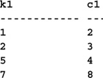
Since Transact-SQL doesn’t include a MEDIAN() aggregate function, computing vector or partitioned medians must be done using something other than the usual GROUP BY technique. Assuming this table and data:
CREATE TABLE #dist (k1 int, c1 int)
INSERT #dist VALUES (1,2)
INSERT #dist VALUES (2,3)
INSERT #dist VALUES (2,1)
INSERT #dist VALUES (2,5)
INSERT #dist VALUES (5,4)
INSERT #dist VALUES (7,8)
INSERT #dist VALUES (7,9)
here’s a modification of the first example to return a vector median:
SELECT d.k1, d.c1
FROM #dist d CROSS JOIN #dist i
WHERE d.k1=i.k1
GROUP BY d.k1, d.c1
HAVING COUNT(CASE WHEN i.c1<=d.c1 THEN 1 ELSE NULL END)=(COUNT(*)+1)/2
ORDER BY d.k1
"K1" is the vectoring or partitioning column in this example. If Transact-SQL had a MEDIAN() aggregate function, “k1” would be the lone item in the GROUP BY list.
A situation that none of the median queries presented thus far handles very well is the presence of duplicate values in the distribution set. In fact, in all of the examples thus far, a duplicate value near the median will cause the query to return NULL or omit the corresponding partition. The problem is that these queries group by the c1 column in the first instance of the work table. Grouping automatically combines duplicate values so that a query cannot distinguish between multiple instances of the same value. Properly handling duplicate values requires the HAVING clause to be reworked. Assuming we start with this table and data:
CREATE TABLE #dist (c1 int)
INSERT #dist VALUES (2)
INSERT #dist VALUES (3)
INSERT #dist VALUES (1)
INSERT #dist VALUES (3) -- Duplicate value
INSERT #dist VALUES (8)
INSERT #dist VALUES (9)
here’s a modification of the statistical median query that handles duplicate values:
SELECT d.c1
FROM #dist d CROSS JOIN #dist i
GROUP BY d.c1
HAVING (COUNT(CASE WHEN i.c1 <= d.c1 THEN 1 ELSE NULL END)>=(COUNT(*)+1)/2)
AND (COUNT(CASE WHEN i.c1 >=d.c1 THEN 1 ELSE NULL END) >= COUNT(*)/2+1)
c1
-----------
3
Likewise, here’s the financial median query modified to handle duplicate values:
CREATE TABLE #dist (c1 int)
INSERT #dist VALUES (2)
INSERT #dist VALUES (2)
INSERT #dist VALUES (1)
INSERT #dist VALUES (5)
INSERT #dist VALUES (5)
INSERT #dist VALUES (9)
SELECT Median=ISNULL((CASE WHEN COUNT(CASE WHEN i.c1<=d.c1 THEN 1 ELSE NULL END)
> (COUNT(*)+1)/2 THEN 1.0*d.c1 ELSE NULL END)+COUNT(*)%2,
(d.c1+MIN((CASE WHEN i.c1>d.c1 THEN i.c1 ELSE NULL END)))/2.0)
FROM #dist d CROSS JOIN #dist i
GROUP BY d.c1
HAVING (COUNT(CASE WHEN i.c1 <= d.c1 THEN 1 ELSE NULL END)>=(COUNT(*)+1)/2)
AND (COUNT(CASE WHEN i.c1 >=d.c1 THEN 1 ELSE NULL END) >= COUNT(*)/2+1)
Median
----------------
3.5
As you can see, things start to get a bit complex when duplicate values enter the picture. Here’s a variation of the financial median query that makes use of a key column (k1) and handles duplicates as well:
CREATE TABLE #dist (k1 int, c1 int)
INSERT #dist VALUES (1,2)
INSERT #dist VALUES (2,2)
INSERT #dist VALUES (3,1)
INSERT #dist VALUES (4,4)
INSERT #dist VALUES (5,5)
INSERT #dist VALUES (6,7)
INSERT #dist VALUES (7,8)
INSERT #dist VALUES (8,9)
SELECT Median=AVG(DISTINCT 1.0*c1)
FROM (SELECT d1.c1
FROM #dist d1 CROSS JOIN #dist d2
GROUP BY d1.k1, d1.c1
HAVING SUM(CASE WHEN d2.c1 = d1.c1 THEN 1 ELSE 0 END) >=
ABS(SUM(CASE WHEN d2.c1 < d1.c1 THEN 1 WHEN d2.c1 > d1.c1 THEN -1 ELSE 0 END))) d
Median
----------------------------------------
4.500000
Clipping is the removal from a set of values a prefix and suffix of some predetermined size. As with medians, figuring out which values to remove is a row-positioning problem—the rows that end up being removed depend on their position in the set. Here’s some sample code that illustrates how easy it is to clip values from a set:
CREATE TABLE #valueset (c1 int)
INSERT #valueset VALUES (2)
INSERT #valueset VALUES (3)
INSERT #valueset VALUES (1)
INSERT #valueset VALUES (4)
INSERT #valueset VALUES (8)
INSERT #valueset VALUES (9)
SELECT v.c1
FROM #valueset v CROSS JOIN #valueset a
GROUP BY v.c1
HAVING v.c1 > MIN(a.c1) AND v.c1 < MAX(a.c1)
c1
-----------
2
3
4
8
This code uses a cross-join and a simple HAVING clause to exclude the minimum and maximum values from the set, but what if we wanted to exclude multiple rows from the beginning or end of the set? We couldn’t simply change > MAX(a.c1) to > MAX(c.c1)+1 because we don’t know whether the values are sequential (in fact, they aren’t, in this case). Accommodating prefix/suffix sizes of more than a single row requires the HAVING clause to be reworked. Here’s a new query that clips prefixes and suffixes of any size:
SELECT v.c1
FROM #valueset v CROSS JOIN #valueset a
GROUP BY v.c1
HAVING COUNT(CASE WHEN a.c1 <=v.c1 THEN 1 ELSE NULL END) > 2
AND COUNT(CASE WHEN a.c1 >= v.c1 THEN 1 ELSE NULL END) >2
c1
-----------
3
4
Note that this code is flexible enough to allow a prefix and a suffix of different sizes. The first predicate in the HAVING clause clips the prefix, and the second clause handles the suffix. The “> 2” comparison construct controls the size of the clipped region. To clip more than two rows, increase the number; to clip less, decrease it.
In SQL Server 7.0 and later, the SELECT statement’s TOP n extension is the most direct way to return a given number of rows from the top or bottom of a result set. TOP n does just what it sounds like—it restricts the rows returned to a specified number. Since you can sort the result set in descending order, TOP n can also return the bottommost rows from a result set. It works similarly to SET ROWCOUNT but can also handle ties and percentages. See the section “SELECT TOP” in Chapter 6 for more information.
If you’re using SQL Server 6.5 or earlier or if you need more flexibility than SELECT TOP n provides, the code from the previous clipping example can be extended to perform a number of useful functions, including returning the topmost or bottommost rows in a result set. One obvious application is to invert it to return a prefix or suffix of a predetermined size. Here’s some sample code that does just that:
SELECT v.c1
FROM #valueset v CROSS JOIN #valueset a
GROUP BY v.c1
HAVING COUNT(CASE WHEN a.c1 >=v.c1 THEN 1 ELSE NULL END) > COUNT(a.c1)-2
c1
-----------
1
2
This code returns the top two rows. As with the previous example, you can modify “-2” to return any number of rows you like. Here’s the same query modified to return the bottom three rows:
SELECT v.c1
FROM #valueset v CROSS JOIN #valueset a
GROUP BY v.c1
HAVING COUNT(CASE WHEN a.c1 <=v.c1 THEN 1 ELSE NULL END) > COUNT(a.c1)-3
c1
-----------
4
8
9
This technique works but has one inherent flaw—it doesn’t handle duplicates. There are a number of solutions to this problem. Here’s one that uses a derived table and a correlated subquery to get the job done:
CREATE TABLE #valueset (c1 int)
INSERT #valueset VALUES (2)
INSERT #valueset VALUES (2) -- Duplicate value
INSERT #valueset VALUES (1)
INSERT #valueset VALUES (3)
INSERT #valueset VALUES (4)
INSERT #valueset VALUES (4) -- Duplicate value
INSERT #valueset VALUES (10)
INSERT #valueset VALUES (11)
INSERT #valueset VALUES (13)
SELECT l.c1
FROM (SELECT ranking=(SELECT COUNT(DISTINCT a.c1) FROM #valueset a
WHERE v.c1 >= a.c1),
v.c1
FROM #valueset v) l
WHERE l.ranking <=3
ORDER BY l.ranking
c1
-----------
1
2
2
3
This technique uses a derived table and a correlated subquery rather than a cross-join to compare #valueset with itself. This, in turn, allows us to get rid of the GROUP BY clause, which caused problems with duplicates. As mentioned earlier, GROUP BY can’t distinguish between multiple instances of the same value. When duplicate values exist within its grouping column(s), it combines them. The key, then, is to return all the rows in #valueset filtered by criteria that restrict them based on their rank among the other values.
The above code uses a derived table to yield a list of rankings for the values in #valueset. This derived table uses a correlated subquery to rank each value according to the number of other values in the table that are less than or equal to it. The subquery is “correlated” because it relates to (in this case, is filtered by) values in the outer table. (Note the use of v alias in the SELECT COUNT(DISTINCT query.) Those with a rank of three or better make the cut.
Note that you can easily alter this query to return the bottommost rows in the set rather than the topmost. Here’s the query modified to return the bottom four rows from the table:
CREATE TABLE #valueset (c1 int)
INSERT #valueset VALUES (2)
INSERT #valueset VALUES (2) -- Duplicate value
INSERT #valueset VALUES (1)
INSERT #valueset VALUES (3)
INSERT #valueset VALUES (4)
INSERT #valueset VALUES (4) -- Duplicate value
INSERT #valueset VALUES (11)
INSERT #valueset VALUES (11) -- Duplicate value
INSERT #valueset VALUES (13)
SELECT l.c1
FROM (SELECT ranking=(SELECT COUNT(DISTINCT a.c1) FROM #valueset a
WHERE v.c1 <= a.c1),
v.c1
FROM #valueset v) l
WHERE l.ranking <=4
ORDER BY l.ranking
c1
-----------
13
11
11
4
4
3
Note that both of these queries allow ties in the result set, so you may get back more rows than you request. If this is undesirable, you can use SELECT TOP or SET ROWCOUNT to limit the actual number of rows returned, as the examples that follow illustrate.
Another alternative to SELECT’s TOP n extension is the SET ROWCOUNT command. It limits the number of rows returned by a query, so you could do something like this in order to return the topmost rows from a result set:
Returning the Bottom n Rows is equally simple. To return the bottommost rows instead of the topmost, change the ORDER BY to sort in descending order.
While this solution is certainly straightforward, it can’t handle duplicates very flexibly. You get exactly three rows, no more, no less. Ties caused by duplicate values are not handled differently from any other value. If you request three rows and there’s a tie for second place, you won’t actually see the real third place row—you’ll see the row that tied for second place in the third slot instead. This may be what you want, but if it isn’t, there is a variation of this query that deals sensibly with ties. It takes advantage of the fact that assigning a variable using a query that returns more than one row assigns the value from the last row to the variable. This is a rarely used trick, and you should probably comment your code to indicate that it’s actually what you intended to do. Here’s the code:
CREATE TABLE #valueset (c1 int)
INSERT #valueset VALUES (2)
INSERT #valueset VALUES (2) -- Duplicate value
INSERT #valueset VALUES (1)
INSERT #valueset VALUES (3)
INSERT #valueset VALUES (4)
INSERT #valueset VALUES (4) -- Duplicate value
INSERT #valueset VALUES (11)
INSERT #valueset VALUES (11) -- Duplicate value
INSERT #valueset VALUES (13)
DECLARE @endc1 int
-- Get third distinct value
SELECT DISTINCT TOP 3 @endc1=c1 FROM #valueset ORDER BY c1
SELECT * FROM #valueset WHERE c1 <= @endc1 ORDER BY c1
c1
-----------
1
2
2
3
This query uses DISTINCT to avoid being fooled by duplicates. Without it, the query wouldn’t handle duplicates any better than its predecessor. What we want to do here is assign the value of the third distinct value to our control variable so that we can then limit the rows returned by the ensuing SELECT to those with values less than or equal to it. So, if there are duplicates in the top three values, we’ll get them. If there aren’t, no harm done—the query still works as expected.
Closely related to the Top n Rows problem is that of producing rankings for a set of data. In fact, you’ll note that one of the Top n Rows solutions used a ranking column to qualify the rows it returned. Here’s that query again with the ranking column included in the SELECT list:
CREATE TABLE #valueset (c1 int)
INSERT #valueset VALUES (2)
INSERT #valueset VALUES (2) -- Duplicate value
INSERT #valueset VALUES (1)
INSERT #valueset VALUES (3)
INSERT #valueset VALUES (4)
INSERT #valueset VALUES (4) -- Duplicate value
INSERT #valueset VALUES (11)
INSERT #valueset VALUES (11) -- Duplicate value
INSERT #valueset VALUES (13)
SELECT l.ranking, l.c1
FROM (SELECT ranking=(SELECT COUNT(DISTINCT a.c1) FROM #valueset a
WHERE v.c1 <= a.c1),
v.c1
FROM #valueset v) l
ORDER BY l.ranking
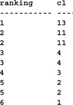
This query isn’t as efficient as it might be since the correlated subquery is executed for every row in #valueset. Here’s a more efficient query that yields the same result:
SELECT Ranking=IDENTITY(int), c1
INTO #rankings
FROM #valueset
WHERE 1=2 -- Create an empty table
INSERT #rankings (c1)
SELECT c1
FROM #valueset
ORDER BY c1 DESC
SELECT * FROM #rankings ORDER BY Ranking
DROP TABLE #rankings

Note the use of SELECT...INTO to create the temporary working table. It uses the IDENTITY() function to create the table en passant rather than explicitly via CREATE TABLE. Though CREATE TABLE would have been syntactically more compact in this case, I think it’s instructive to see how easily SELECT...INTO allows us to create work tables.
The SELECT...INTO is immediately followed by an INSERT that populates it with data. Why not perform the two operations in one pass? That is, why doesn’t the SELECT...INTO move the data into the #rankings table at the same time that it creates it? There are two reasons. First, SELECT...INTO is a special nonlogged operation that locks system tables while it runs, so initiating one that could conceivably run for an extended period of time is a bad idea. In the case of tempdb, you’ll block other users creating temporary tables, possibly prompting them to tar and feather you. Second, SQL Server doesn’t work as expected here—it hands out identity values based on the natural order of the #valueset table rather than according to the query’s ORDER BY clause. So, even if locking the system tables wasn’t a concern, this anomaly in SQL Server’s row ordering would prevent us from combining the two steps anyway.
This query doesn’t handle ties as you might expect. Since the items in the #rankings table are numbered sequentially, values that are actually duplicates (and hence tied) are listed in sequence as though no tie existed. If you restrict the rows returned to a given segment of the top of the list and ties are present, you won’t get the results you may be expecting. For example, if you ask for four rows and there was a tie for second, you’ll only see the row in first place followed by the two that tied for second and the one that placed third. You won’t actually see the fourth place row. Since there’s no way to know how many ties you might have, returning the top four rankings from the set is more involved than it probably should be, but modifying the query to rank the rows more sensibly is fairly easy. Here’s an example:
SELECT Ranking=IDENTITY(int), c1
INTO #rankings
FROM #valueset
WHERE 1=2 -- Create an empty table
INSERT #rankings (c1)
SELECT c1
FROM #valueset
ORDER BY c1 DESC
SELECT a.Ranking, r.c1
FROM
(SELECT Ranking=MIN(n.Ranking), n.c1 FROM #rankings n GROUP BY n.c1) a,
#rankings r
WHERE r.c1=a.c1
ORDER BY a.ranking
DROP TABLE #rankings
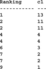
In this query, ties are indicated by identical rankings. In the case of our earlier example, the two rows tied for second place would be ranked second, followed by the third row, which would be ranked fourth. This is the way that ties are often handled in official rankings; it keeps the number of values above a particular ranking manageable.
One piece of information that’s missing from the above query is an indication of which rows are ties and how many ties exist for each value. Here’s a modification of the query that includes this information as well:
SELECT a.Ranking, Ties=CAST(LEFT(CAST(a.NumWithValue AS varchar)+'-Way tie',
NULLIF(a.NumWithValue,1)*11) AS CHAR(11)), r.c1
FROM
(SELECT Ranking=MIN(n.Ranking), NumWithValue=COUNT(*), n.c1 FROM #rankings n
GROUP BY n.c1) a,
#rankings r
WHERE r.c1=a.c1
ORDER BY a.ranking
DROP TABLE #rankings

There are three basic ways to reflect a middle or typical value for a distribution of values: medians, means (averages), and modes. We’ve already covered medians and averages, so let’s explore how to compute the mode of a set of values. A distribution’s mode is its most common value, regardless of where the value physically appears in the set. If you have this set of values:
10, 10, 9, 10, 10
the mode is 10, the median is 9, and the mean is 9.8. The mode is 10 because it’s obviously the most common value in the set. Here’s a Transact-SQL query that computes the mode for a more complex set of values:
CREATE TABLE #valueset (c1 int)
INSERT #valueset VALUES (2)
INSERT #valueset VALUES (2)
INSERT #valueset VALUES (1)
INSERT #valueset VALUES (3)
INSERT #valueset VALUES (4)
INSERT #valueset VALUES (4)
INSERT #valueset VALUES (10)
INSERT #valueset VALUES (11)
INSERT #valueset VALUES (13)
SELECT TOP 1 WITH TIES c1, COUNT(*) AS NumInstances
FROM #valueset
GROUP BY c1
ORDER BY NumInstances DESC

Since a set may have more than one value with the same number of occurrences, it’s possible that there may be multiple values that qualify as the set’s mode. That’s where SELECT’s TOP n extension comes in handy. Its WITH TIES option can handle situations like this without requiring additional coding.
The CASE function makes computing certain types of histograms quite easy, especially horizontal histograms. Using a technique similar to that in the pivoting example earlier in the chapter, we can build horizontal histogram tables with a trivial amount of Transact-SQL code. Here’s an example that references the sales table in the pubs database:
SELECT
"Less than 10"=COUNT(CASE WHEN s.sales >=0 AND s.sales <10 THEN 1 ELSE NULL END),
"10-19"=COUNT(CASE WHEN s.sales >=10 AND s.sales <20 THEN 1 ELSE NULL END),
"20-29"=COUNT(CASE WHEN s.sales >=20 AND s.sales <30 THEN 1 ELSE NULL END),
"30-39"=COUNT(CASE WHEN s.sales >=30 AND s.sales <40 THEN 1 ELSE NULL END),
"40-49"=COUNT(CASE WHEN s.sales >=40 AND s.sales <50 THEN 1 ELSE NULL END),
"50 or more"=COUNT(CASE WHEN s.sales >=50 THEN 1 ELSE NULL END)
FROM (SELECT t.title_id, sales=ISNULL(SUM(s.qty),0) FROM titles t LEFT OUTER JOIN sales
s ON (t.title_id=s.title_id) GROUP BY t.title_id) s
![]()
The query computes the titles that fall into each group based on their sales. Note the use of a derived table to compute the sales for each title. This is necessary because the COUNT() expressions in the SELECTs column list cannot reference other aggregates. Once the sales for each title are computed, this number is compared against the range for each group to determine its proper placement.
Histograms have a tendency to make obscure trends more obvious. This particular one illustrates that most titles have sold between ten and thirty copies.
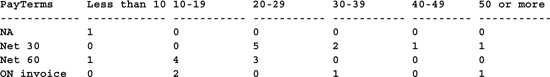
Beyond simple histograms, stratified histograms are crucial to comparative statistical analysis. They allow data to be compared in multiple dimensions—both horizontally and vertically. Here’s a modification of the first histogram example to include a stratification column:
SELECT
PayTerms=isnull(s.payterms,'NA'),
"Less than 10"=COUNT(CASE WHEN s.sales >=0 AND s.sales <10 THEN 1 ELSE NULL END),
"10-19"=COUNT(CASE WHEN s.sales >=10 AND s.sales <20 THEN 1 ELSE NULL END),
"20-29"=COUNT(CASE WHEN s.sales >=20 AND s.sales <30 THEN 1 ELSE NULL END),
"30-39"=COUNT(CASE WHEN s.sales >=30 AND s.sales <40 THEN 1 ELSE NULL END),
"40-49"=COUNT(CASE WHEN s.sales >=40 AND s.sales <50 THEN 1 ELSE NULL END),
"50 or more"=COUNT(CASE WHEN s.sales >=50 THEN 1 ELSE NULL END)
FROM (SELECT t.title_id, s.payterms, sales=ISNULL(SUM(s.qty),0) FROM titles t LEFT OUTER JOIN sales s ON (t.title_id=s.title_id) GROUP BY t.title_id, payterms) s
GROUP BY s.payterms
Histograms, pivot tables, and other types of OLAP constructs can also be built using SQL Server’s OLAP Services module. Coverage of this suite of tools is outside the scope of this book, so you should consult the Books Online for further information.
Computing running totals in Transact-SQL is relatively straightforward. As in many of the other examples in this chapter, the technique presented here makes use of a cross-join between two copies of the source table. Here’s the code:
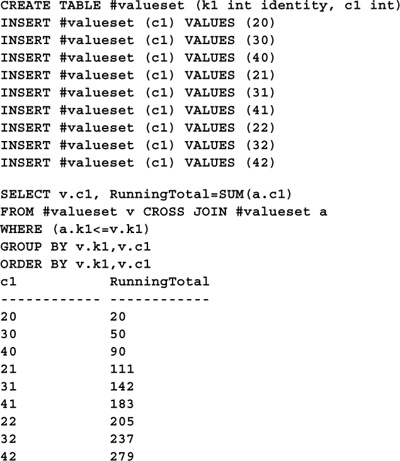
Note the inclusion of the ORDER BY clause. It’s required because the GROUP BY clause does not implicitly order the result set as it did in earlier releases of SQL Server.
Other types of running aggregates can be computed by replacing SUM()with another aggregate function. For example, to compute a running AVG(), try this:

To compute a running count (which produces unique row numbers), try this:

A sliding aggregate differs from a cumulative aggregate in that it reflects an aggregation of a sequence of values around each value in a set. This subset “moves” or “slides” with each value, hence the term. So, for example, a sliding average might compute the average of the current value and its preceding four siblings, like so:

Note that the sliding averages for the first four values are returned as running averages since they don’t have the required number of preceding values. Beginning with the fifth value, though, SlidingAverage reflects the mean of the current value and the four immediately before it. As with the running totals example, you can replace AVG() with different aggregate functions to compute other types of sliding aggregates.
An extreme, as defined here, is the largest value among two or more columns in a given table. You can think of it as a horizontal aggregate. Oracle has functions (GREATEST() and LEAST()) to return horizontal extremes; Transact-SQL doesn’t. However, retrieving a horizontal extreme value for two columns is as simple as using CASE to select between them, like so:
CREATE TABLE #tempsamp
(SampDate datetime,
Temp6am int,
Temp6pm int)
INSERT #tempsamp VALUES ('19990101',44,32)
INSERT #tempsamp VALUES ('19990201',41,39)
INSERT #tempsamp VALUES ('19990301',48,56)
INSERT #tempsamp VALUES ('19990401',65,72)
INSERT #tempsamp VALUES ('19990501',59,82)
INSERT #tempsamp VALUES ('19990601',47,84)
INSERT #tempsamp VALUES ('19990701',61,92)
INSERT #tempsamp VALUES ('19990801',56,101)
INSERT #tempsamp VALUES ('19990901',59,78)
INSERT #tempsamp VALUES ('19991001',54,74)
INSERT #tempsamp VALUES ('19991101',47,67)
INSERT #tempsamp VALUES ('19991201',32,41)
SELECT HiTemp=CASE WHEN Temp6am > Temp6pm THEN Temp6am ELSE Temp6pm END
FROM #tempsamp
HiTemp
-----------
44
41
56
72
82
84
92
101
78
74
67
41
You can nest CASE functions within one another if there are more than two horizontal values to consider.
Note that you can also order result sets using extreme values. All that’s necessary is to reference the CASE function’s column alias in the ORDER BY clause like this:
SELECT HiTemp=CASE WHEN Temp6am > Temp6pm THEN Temp6am ELSE Temp6pm END
FROM #tempsamp
ORDER BY HiTemp
HiTemp
-----------
41
41
44
56
67
72
74
78
82
84
92
101
If you wish to order by the extreme without actually selecting it, simply move the CASE expression from the SELECT list to the ORDER BY clause. Here’s a query that returns the samples sorted by the lowest temperature on each sample date:
SELECT *
FROM #tempsamp
ORDER BY CASE WHEN Temp6am < Temp6pm THEN Temp6am ELSE Temp6pm END

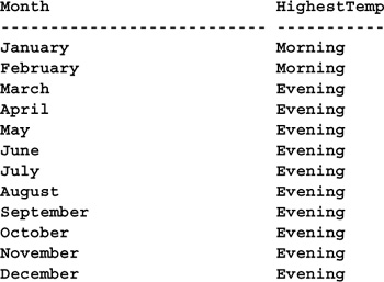
Beyond returning horizontal extreme values, a query might need to indicate which attribute actually contains the extreme value. Here’s a query that does that:
SELECT Month=DATENAME(mm,SampDate),
HighestTemp=CASE WHEN Temp6am > Temp6pm THEN 'Morning' ELSE 'Evening' END
FROM #tempsamp
Once you’ve computed a horizontal extreme, you may wish to find all the rows in the table with the same extreme value. You can do this using CASE in conjunction with a subquery. Here’s an example:

In this chapter, you learned about computing statistical information using Transact-SQL. You learned about the built-in statistical functions as well as how to build your own. Thanks to SQL Server’s set orientation and statistical functions, it’s a very capable statistics calculation engine—more so, in fact, than many 3GL tools.