
9 Runs and Sequences
I like to remind my team that ultimately we ship products, not specs and design documents, so we need to remember the end game.—Ron Soukup
Runs, regions, sequences, and series are related data constructs that usually include a minimum of two columns: a key column that is more or less sequential and a value column that contains the information in which we’re interested. The key column of a sequence (or series) is sequential, with no gaps between identifiers. Examples of sequences include time series, invoice numbers, account numbers, and so on. A run’s key column is also sequential, though there may or may not be gaps between identifiers. Examples of runs include those of regular sequences (with gaps, of course) as well as house numbers, version numbers, and the like. A region is a subsequence whose members all meet the same criteria. The simplest example of a region is a subsequence whose members all have the same value. An interval is the product of dividing a sequence or run into multiple, evenly sized subsequences or subsets.
Queries to process these constructs are often quite similar to one another, and the techniques to process one type of ordered list may overlap those of another. So, the query that finds relationships between the members of a run may also work with time series data—it just depends on what you’re doing.
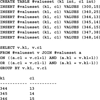
Time series are probably the most ubiquitous examples of sequences. A common need with time series is to find areas or periods within a series where values have a particular relationship to one another. You might want to know, for example, the range of time when a stock issue was steadily increasing in price, when prices were within a certain percentage of one another, and so on. Here’s a query that demonstrates how to do this in Transact-SQL:

This query identifies regions within the series where values increase in succession. It uses a self-join to compare the work table with itself, then removes duplicates from the result set via a GROUP BY clause. Note the use of the DATEADD() function to refer to each data point’s next and previous months.
Another common need with time series is to compute the change from one value to the next. You can use this measurement to gauge volatility from point to point within the series and to identify outlying values. Here’s an example:

There are several interesting elements here worth mentioning. First, note the use of derived tables to rank the values in the series against one another. Though it would be syntactically more compact to move these to a view, this approach demonstrates the viability of a single SELECT to get at the data we want.
Next, note the use of a subquery within each derived table to compute the ranking itself. It does this via a COUNT(DISTINCT) of the other values in the work table that are less than or equal to each value. Finally, note the use of the SIGN() and SUBSTRING() functions to produce a sign prefix for each change. While simply displaying a.c1-v.c1 would have indicated negative changes via the standard “–” prefix, positive changes would have remained unsigned.
Performing calculations or computing statistics on every nth value is another common sequence-related task. Because the query above materializes the rankings of each item in the time series, this is relatively trivial to do. Here’s the earlier query modified to sample every third value:

The only real change here is the use of modulus 3 to qualify the rows the query returns. Since only third rows will satisfy v.ranking%3, we get the result we’re after.
The most common region-related task is identifying the regions in the first place. Unlike sequences and runs, where the presence of the construct itself is implicit, a region is defined by its values. Members of a particular region are sequential, and all meet the same membership criteria. These criteria may stipulate that all members of the region have the same absolute value, that each value has the same relationship to the previous value, or that each value qualifies in some other way. Here’s a technique for identifying regions within a sequence:
CREATE TABLE #valueset (k1 int identity, c1 int)
INSERT #valueset (c1) VALUES (20)
INSERT #valueset (c1) VALUES (30)
INSERT #valueset (c1) VALUES (0)
INSERT #valueset (c1) VALUES (0)
INSERT #valueset (c1) VALUES (0)
INSERT #valueset (c1) VALUES (41)
INSERT #valueset (c1) VALUES (0)
INSERT #valueset (c1) VALUES (32)
INSERT #valueset (c1) VALUES (42)
SELECT v.k1
FROM #valueset v JOIN #valueset a
ON (v.c1=0) AND (a.c1=0) AND (ABS(a.k1-v.k1)=1)
GROUP BY v.k1
k1
-----------
3
4
5
As illustrated here, the region consists of items in the sequence whose value is zero. The query’s magic is performed via a self-join that’s filtered for duplicates via the GROUP BY clause. The ON clause limits the values considered to 1) those whose value is zero and 2) those with an adjacent value of zero. Adjacency is determined by subtracting the value of the key column in v from that of a. An absolute value of one indicates that the key is either just before or just after the one in v.
In addition to absolute values, relative conditions are a popular criterion for establishing region membership. A relative condition identifies some relationship between the values in the sequence. Finding regions whose values increase sequentially is an example of finding a region based on a relative condition. Here’s some Transact-SQL code that identifies a region whose values increase monotonically:
Again, we use a self-join to compare the work table with itself. The two join criteria established by the ON clause are 1) each key value in the region must be one less or one more than the value under consideration and 2) each value must be correspondingly sequential with its adjacent values.
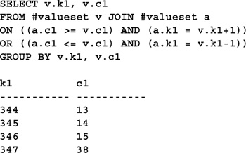
Note that it’s not difficult to modify this query to look for values that merely increase from point to point in the series—that is, ones that aren’t necessarily contiguous. Here’s an example:
Once we’ve identified a region, it may be desirable to qualify it further based on size. We may not want to see within a sequence every region whose members have an absolute value or have a specific relationship to one another—we may want to limit the regions we consider to those of a particular size or larger. Here’s some Transact-SQL code that illustrates how to constrain regions based on size:
CREATE TABLE #valueset(k1 int identity, c1 int)
INSERT #valueset(c1) VALUES (20)
INSERT #valueset(c1) VALUES (30)
INSERT #valueset(c1) VALUES (32)
INSERT #valueset(c1) VALUES (34)
INSERT #valueset(c1) VALUES (36)
INSERT #valueset(c1) VALUES (0)
INSERT #valueset(c1) VALUES (0)
INSERT #valueset(c1) VALUES (41)
INSERT #valueset(c1) VALUES (0)
INSERT #valueset(c1) VALUES (0)
INSERT #valueset(c1) VALUES (0)
INSERT #valueset(c1) VALUES (42)
SELECT v.k1
FROM #valueset v JOIN #valueset a ON (v.c1=0)
GROUP BY v.k1
HAVING
(ISNULL(MIN(CASE WHEN a.k1 > v.k1 AND a.c1 !=0 THEN a.k1 ELSE null END)-1,
MAX(CASE WHEN a.k1 > v.k1 THEN a.k1 ELSE v.k1 END))
-
ISNULL(MAX(CASE WHEN a.k1 < v.k1 AND a.c1 !=0 THEN a.k1 ELSE null END)+1,
MIN(CASE WHEN a.k1 < v.k1 THEN a.k1 ELSE v.k1 END)))+1
>=3 -- Desired region size
The “>=3” above constrains the size of the regions listed to those of three or more elements, as the code comment indicates. Note how the first region (consisting of two zero values) in the series is ignored by the query since it’s too small. Only the second one, which has the required number of members, is returned.
Beyond the use of JOIN and GROUP BY to compare the table with itself, the real work of the query is performed by the HAVING clause. Consider the first ISNULL() expression. It uses CASE to find either 1) the first key in a that is both less than the current key in v and whose value is nonzero or 2) the last key in a that is greater than the current key in v. If a key that meets the first criterion isn’t found, it will always be the last key in the table. The idea is to find the nearest nonzero value following the current key in v. What we are attempting to do is identify the key value of the region’s lower boundary—its terminator.
The second ISNULL() expression is essentially a mirror image of the first. Its purpose is to establish the identity of the first key in the region. Once the boundary keys have been identified, the upper boundary is subtracted from the lower boundary to yield the region size. This is then compared to “>=3” to filter out regions smaller than three members in size.
Though this technique works and is relatively compact from a coding standpoint, I’d be the first to concede that, at least on the surface, it appears to be a bit convoluted. For example, CASE is used to “throw” a NULL back to ISNULL()—which forces ISNULL() to evaluate its second argument—forming a crude nested if-then-else expression. Written a bit more clearly, the first ISNULL() expression might look like this:
CASE
WHEN a.k1 > v.k1 AND a.c1 !=0 THEN MIN(a.k1)-1
ELSE MAX(CASE WHEN a.k1 > v.k1 THEN a.k1 ELSE v.k1 END)
END
The problem with this is that the plain references to a.k1 and a.c1 aren’t allowed in the HAVING clause because they aren’t contained in either an aggregate or the GROUP BY clause. This is an ANSI SQL restriction and is normally a good thing—except when you’re attempting complex queries with single SELECTs like this one. We can’t do much about the fact that they aren’t in the GROUP BY clause—we need to leave it as is to consolidate our self-join. However, we can nest both of these values within aggregate functions so that they conform to ANSI SQL’s HAVING clause restrictions. And this is exactly what the query does—it “hides” CASE function logic within aggregates to get past limitations imposed by HAVING—and it’s the main reason the logic appears somewhat tangled at first.
Like their contiguous sequence cousins, runs include a minimum of two columns: a key column and a value column. The key column is always sequential, though its values may not be contiguous.
As with sequences, the existence of a run is implicit. Examples of runs include time series with irregular entry points and numbering systems with gaps (e.g., invoice numbers, credit card numbers, house numbers).
By contrast, regions within runs are not implicit. As described earlier, regions exist based on membership. The Transact-SQL code required to locate regions within a run is not unlike that used to find them within sequences. Here’s an example:
CREATE TABLE #valueset (k1 int, c1 int)
INSERT #valueset VALUES (2,0)
INSERT #valueset VALUES (3,30)
INSERT #valueset VALUES (5,0)
INSERT #valueset VALUES (9,0)
INSERT #valueset VALUES (10,0)
INSERT #valueset VALUES (11,40)
INSERT #valueset VALUES (13,0)
INSERT #valueset VALUES (14,0)
INSERT #valueset VALUES (15,42)
SELECT v.k1
FROM #valueset v JOIN #valueset a ON (v.c1=0)
GROUP BY v.k1
HAVING (MIN(CASE WHEN a.k1 > v.k1 THEN (2*(a.k1-v.k1))+CASE WHEN a.c1<>0 THEN 1
ELSE 0 END ELSE null END)%2=0)
OR (MIN(CASE WHEN a.k1 < v.k1 THEN (2*(v.k1-a.k1))+CASE WHEN a.c1<>0 THEN 1 ELSE
0 END ELSE null END)%2=0)
As with many of the other queries, this query uses a self-join/GROUP BY combo to compare the work table with itself. Note the use of nested CASE expressions to effect some fairly complex logic. Also note the way in which this logic is wrapped within aggregate functions so that it complies with ANSI SQL’s restrictions on the HAVING clause.
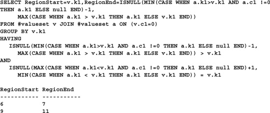
As we did with sequences, let’s explore how to return the outer boundaries of run regions rather than the regions themselves. Here’s some code that returns the boundaries of the regions it encounters within a run:
CREATE TABLE #valueset (k1 int, c1 int)
INSERT #valueset VALUES (2,20)
INSERT #valueset VALUES (3,30)
INSERT #valueset VALUES (5,0)
INSERT #valueset VALUES (9,0)
INSERT #valueset VALUES (10,0)
INSERT #valueset VALUES (11,40)
INSERT #valueset VALUES (13,0)
INSERT #valueset VALUES (15,0)
INSERT #valueset VALUES (16,42)
SELECT StartRun=v.k1, EndRun=a.k1
FROM #valueset v JOIN #valueset a ON (v.k1 < a.k1) CROSS JOIN #valueset l
GROUP BY v.k1, a.k1
HAVING
(SUM(ABS(l.c1)*(CASE WHEN v.k1 <=l.k1 AND l.k1 <= a.k1 THEN 1 ELSE 0 END))=0)
AND (ISNULL(MIN(CASE WHEN l.k1 > a.k1
THEN (2*(l.k1-a.k1))+(CASE WHEN l.c1<>0 THEN 1 ELSE 0 END)
ELSE null END),1)%2 != 0)
AND (ISNULL(MIN(CASE WHEN l.k1 < v.k1
THEN (2*(v.k1-l.k1))+(CASE WHEN l.c1<>0 THEN 1 ELSE 0 END)
ELSE null END),1)
%2 != 0)
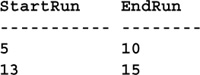
As with the previous query, this example embeds much of its work within aggregate functions in the HAVING clause. Some of this is counterintuitive. Note, for example, the HAVING clause expression:
(SUM(ABS(l.c1)*(CASE WHEN v.k1 <=l.k1 AND l.k1 <= a.k1 THEN 1 ELSE 0 END)) =0)
Written more legibly, it might read:
((CASE WHEN v.k1 <=l.k1 AND l.k1 <= a.k1 THEN SUM(ABS(l.c1)) ELSE 0 END)50)
However, as mentioned before, v.k1 and l.k1 must either also appear in the GROUP BY clause or be wrapped in an aggregate function in order to be used in the HAVING clause, so this syntax won’t work. Instead, we return either one or zero from the CASE expression and then multiply SUM(ABS(l.c1)) by it, achieving the same result.
Another interesting characteristic of this query is the use of three instances of the work table. The fact that the run’s key values may not be sequential causes some additional work that requires a third instance of the table to be performed, even though no columns are returned from it by the query.
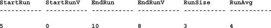
As mentioned in the sequence examples, the need to constrain regions based on size is a common one. Here’s a Transact-SQL query that scans a run for regions consisting of three or more members with values less than 10:
CREATE TABLE #valueset (k1 int, c1 int)
INSERT #valueset VALUES (2,20)
INSERT #valueset VALUES (3,30)
INSERT #valueset VALUES (5,0)
INSERT #valueset VALUES (9,4)
INSERT #valueset VALUES (10,8)
INSERT #valueset VALUES (11,40)
INSERT #valueset VALUES (13,0)
INSERT #valueset VALUES (15,12)
INSERT #valueset VALUES (16,42)
SELECT
StartRun=v.k1,
StartRunV=v.c1,
EndRun=a.k1,
EndRunV=a.c1,
RunSize=COUNT(CASE WHEN v.k1 <= l.k1 AND l.k1 <= a.k1 THEN 1 ELSE null END),
RunAvg=AVG(CASE WHEN v.k1 <= l.k1 AND l.k1 <= a.k1 THEN l.c1 ELSE null END)
FROM #valueset v JOIN #valueset a ON (v.k1 < a.k1) CROSS JOIN #valueset l
GROUP BY v.k1, v.c1, a.k1, a.c1
HAVING (COUNT(CASE WHEN v.k1 <= l.k1 AND l.k1 <= a.k1 THEN 1 ELSE NULL END)>=3)
-- 3 = Desired Run size
AND (COUNT((CASE WHEN l.c1 >=10 THEN 1 ELSE NULL END)*(CASE WHEN v.k1 <= l.k1 AND l.k1 <= a.k1 THEN 1 ELSE NULL END))=0)
AND (ISNULL(MIN((CASE WHEN l.k1 > a.k1 THEN (2*(l.k1-a.k1))+(CASE WHEN l.c1>=10 THEN 1 ELSE 0 END) ELSE null END)),1)%2 != 0)
AND (ISNULL(MIN((CASE WHEN l.k1 < v.k1 THEN (2*(v.k1-l.k1))+(CASE WHEN l.c1>=10 THEN 1 ELSE 0 END) ELSE null END)),1)%2 != 0)
This query also requires three instances of the work table to get the job done. It self-joins the first two, then cross-joins the third and removes the resulting duplicates using a GROUP BY clause. Beyond that, most of the logic controlling which rows make it into the result set is contained in the HAVING clause. As in many of the examples presented thus far, much of the selection logic is embedded in aggregate functions so that it conforms to the restrictions imposed by HAVING.
An interval is an ordered subsequence of values of a particular size. The ability to split a sequence into a given number of equally sized intervals has lots of business applications—everything from stratifying customer lists to breaking sample sequences into more manageable chunks. Assuming we start with the following table:
CREATE TABLE #valueset (c1 int)
INSERT #valueset VALUES (20)
INSERT #valueset VALUES (30)
INSERT #valueset VALUES (40)
INSERT #valueset VALUES (21)
INSERT #valueset VALUES (31)
INSERT #valueset VALUES (41)
INSERT #valueset VALUES (22)
INSERT #valueset VALUES (32)
INSERT #valueset VALUES (42)
here’s a Transact-SQL SELECT statement that breaks the sequence into three intervals, returning the end point of each one:
SELECT v.c1
FROM #valueset v CROSS JOIN #valueset a
GROUP BY v.c1
HAVING COUNT(CASE WHEN a.c1 <= v.c1 THEN 1 ELSE null END)%(COUNT(*)/3)=0
c1
-----------
22
32
42
Here again we use the JOIN/GROUP BY combo to compare the table with itself. And, again, the query’s selection logic is embedded in its HAVING clause. The “/3” in the HAVING clause indicates the interval size we seek. The HAVING clause works by counting the number of items in a that are less than or equal to the current item in v, then checking that number modulus the total number of rows divided by the desired interval size. If the modulus is zero, we have an interval end point that will be returned by the query.
Note that it’s trivial to return the position of each end point as well. Here’s the code:

To get the start points rather than the end points of each interval, change the modulus check to “1,” like this:
SELECT v.c1
FROM #valueset v CROSS JOIN #valueset a
GROUP BY v.c1
HAVING COUNT(CASE WHEN a.c1 <= v.c1 THEN 1 ELSE null END)%(COUNT(*)/3)=1
c1
-----------
20
30
40
Rather than computing intervals over an entire sequence, it’s often desirable to compute them in a sectioned or partitioned fashion. That is, instead of seeing all the partitions across an entire table, we might want to see them grouped based on a particular column—a GROUP BY column (or columns), if you will. Since Transact-SQL has no INTERVAL_BEGIN()- or INTERVAL_END()-type aggregate functions, performing a vector computation such as this requires a nontraditional approach. As with most of the solutions presented in this chapter, the technique presented here uses the Cartesian product of two instances of the work table, together with GROUP BY and HAVING to return the data we seek. Here’s a Transact-SQL routine that returns a partitioned listing of interval information:
CREATE TABLE #valueset (k1 int, c1 int)
INSERT #valueset VALUES (1,20)
INSERT #valueset VALUES (1,21)
INSERT #valueset VALUES (1,22)
INSERT #valueset VALUES (1,24)
INSERT #valueset VALUES (1,28)
INSERT #valueset VALUES (2,31)
INSERT #valueset VALUES (2,32)
INSERT #valueset VALUES (2,40)
INSERT #valueset VALUES (2,41)
INSERT #valueset VALUES (3,52)

This code partitions, or groups, the rows in the table using the k1 column into intervals of four. It then returns the top two values from each interval. This would be useful, for example, if you needed to return the top n salespeople from each region or the top n students within each class, but you wanted to constrain the list to intervals of a particular size to filter out salespeople in regions with no competition or students in classes with few other students.
Sequences, series, runs, and regions are similar data constructs that typically include at least two columns: a sequential (though not necessarily contiguous) key column and a value column. Sequences and series are synonymous. A sequence’s key column values are sequential, with no gaps between them. A run’s key column values are also sequential, though they may not be contiguous. A region is a portion of a sequence or run whose members meet a given set of criteria. Intervals are produced by dividing a sequence or run into multiple, evenly sized subsequences or subsets.
In this chapter, you learned how to use self-joins and cross-joins to identify complex data trends and data relationships within tables. Using the example code included in this chapter, you should be able to solve most types of run- and sequence-related problems without resorting to control-of-flow language statements such as loops.