
Keras is an open source neural network library that is written in Python. It focuses on being minimal, modular, and extensible, and was designed in order to enable fast experimentation with DNNs.
This library, whose primary author and maintainer is a Google engineer named François Chollet, was developed as part of the research effort of project ONEIROS (Open-ended Neuro-Electronic Intelligent Robot Operating System).
Keras was developed following these design principles:
- Modularity: A model is understood as a sequence or a graph of standalone, fully-configurable modules that can be plugged together with as few restrictions as possible. Neural layers, cost functions, optimizers, initialization schemes, and activation functions are all standalone modules that can be combined to create new models.
- Minimalism: Each module must be short (a few lines of code) and simple. The source code should be transparent upon the dirt reading.
- Extensibility: New modules are simple to add (like new classes and functions), and existing modules provide examples on which to base new modules. Being able to easily create new modules allows total expressiveness, making Keras suitable for advanced research.
Keras, is available both in the embedded version as a TensorFlow API, and as a library:
- tf.keras from https://www.tensorflow.org/api_docs/python/tf/keras
- Keras v 2.1.4 (please see at https://keras.io for updates and installation guide)
In the following sections we will see how to use both the first and the second implementation.
The core data structure of Keras is a model, which is a way to organize layers. There are two types of model:
In this section, we'll quickly explain how sequential models work by showing you the code. Let's start by importing and building the Keras Sequential model using the TensorFlow APIs:
import tensorflow as tf
from tensorflow.python.keras.models import Sequential
model = Sequential()
Once we have defined a model we can add one or more layers. The stacking operation is provided by the add() statement:
from keras.layers import Dense, Activation
For example, let's add a first fully connected neural network layer and the activation function:
model.add(Dense(output_dim=64, input_dim=100))
model.add(Activation("relu"))
Then we add a second softmax layer:
model.add(Dense(output_dim=10))
model.add(Activation("softmax"))
If the model looks fine, we must compile() the model, specifying the loss function and the optimizer to be used:
model.compile(loss='categorical_crossentropy',
              optimizer='sgd',
              metrics=['accuracy'])
We can now configure our optimizer. Keras tries to make programming reasonably simple, allowing the user to be fully in control when they need to.
Once compiled, the model must fit the data:
model.fit(X_train, Y_train, nb_epoch=5, batch_size=32)
Alternatively, we can feed batches to our model manually:
model.train_on_batch(X_batch, Y_batch)
Once it is trained, we can use our model to make predictions on new data:
classes = model.predict_classes(X_test, batch_size=32)
proba = model.predict_proba(X_test, batch_size=32)
In this example, we apply the Keras sequential model to a sentiment analysis problem. Sentiment analysis is the act of deciphering the opinions contained in a written or spoken text. The main purpose of this technique is to identify the sentiment (or polarity) of a lexical expression, which may have a neutral, positive, or negative connotation. The problem that we want to solve is the IMDB movie review sentiment classification problem: each movie review is a variable sequence of words, and the sentiment (positive or negative) of each movie review must be classified.
The problem is very complex because the sequences can vary in length and contain a large vocabulary of input symbols. The solution requires the model to learn long-term dependencies between symbols in the input sequence.
The IMDB dataset contains 25,000 highly polar movie reviews (good or bad) for training, and the same amount again for testing. The data was collected by Stanford researchers and was used in a 2011 paper where a 50-50 split of the data was used for training and testing. In this paper, an accuracy of 88.89% was achieved.
Once we have defined our problem, we are ready to develop a sequential LSTM model to classify the sentiment of movie reviews. We can quickly develop a LSTM for the IMDB problem and achieve good accuracy. Let's start off by importing the classes and functions required for this model and initializing the random number generator to a constant value to ensure we can easily reproduce the results.
In this example we are using the embedded Keras in TensorFlow APIs:
import numpy
from tensorflow.python.keras.models import Sequential
from tensorflow.python.keras.datasets import imdb
from tensorflow.python.keras.layers import Dense
from tensorflow.python.keras.layers import LSTM
from tensorflow.python.keras.layers import Embedding
from tensorflow.python.keras.preprocessing import sequence
numpy.random.seed(7)
We load the IMDB dataset. We are restricting the dataset to the top 5,000 words. We also split the dataset into training (50%) and testing (50%) sets.
Keras provides built-in access to the IMDB dataset. The imdb.load_data() function allows you to load the dataset in a format that is ready for use in neural networks and DL models. The words have been replaced by integers that indicate the ordered frequency of each word in the dataset. The sentences in each review therefore comprise a sequence of integers.
Here's the code:
top_words = 5000
(X_train, y_train), (X_test, y_test) =
                          imdb.load_data(num_words=top_words)
Next, we need to truncate and pad the input sequences so that they are all the same length for modeling. The model will learn the zero values that carry no information, so the sequences are not the same length in terms of content, but the vectors need to be the same length to be computed in Keras. The sequence length in each review varies, so we restricted each review to 500 words, truncating long reviews and padding the shorter reviews with zero values:
Let's see:
max_review_length = 500
X_train = sequence.pad_sequences
                  (X_train, maxlen=max_review_length)
X_test = sequence.pad_sequences
                  (X_test, maxlen=max_review_length)
We can now define, compile, and fit our LSTM model.
To resolve the sentiment classification problem, we'll use the word embedding technique. It consists of representing words in a continuous vector space, which is an area in which the words that are semantically similar are mapped to neighboring points. Word embedding is based on the distributional hypothesis, which states that the words that appear in a given context must share the same semantic meaning. Each movie review will then be mapped into a real vector domain, where the similarity between words in terms of meaning translates to closeness in the vector space. Keras provides a convenient way to convert positive integer representations of words into a word embedding by using an embedding layer.
Here, we define the length of the embedding vector and the model:
embedding_vector_length = 32
model = Sequential()
The first layer is the embedded layer. It uses 32 length vectors to represent each word:
model.add(Embedding(top_words,
                    embedding_vector_length,
                      input_length=max_review_length))
The next layer is the LSTM layer with 100 memory units. Finally, because this is a classification problem, we use a dense output layer with a single neuron and a sigmoid activation function to make predictions about the classes (good and bad) in the problem:
model.add(LSTM(100))
model.add(Dense(1, activation='sigmoid'))
Because it is a binary classification problem, we use binary_crossentropy as the loss function, while the optimizer used here is the adam optimization algorithm (we encountered it in a previous TensorFlow implementation):
model.compile(loss='binary_crossentropy',
              optimizer='adam',
                metrics=['accuracy'])
print(model.summary())
We only fit three epochs, because the model quickly overfits. A batch size of 64 reviews is used to space out weight updates:
model.fit(X_train, y_train,
           validation_data=(X_test, y_test),
              num_epochs=3,
                batch_size=64)
Then, we estimate the model's performance on unseen reviews:
scores = model.evaluate(X_test, y_test, verbose=0)
print("Accuracy: %.2f%%" % (scores[1]*100))
Running this example produces the following output:
Epoch 1/3
16750/16750 [==============================] - 107s - loss: 0.5570 - acc: 0.7149
Epoch 2/3
16750/16750 [==============================] - 107s - loss: 0.3530 - acc: 0.8577
Epoch 3/3
16750/16750 [==============================] - 107s - loss: 0.2559 - acc: 0.9019
Accuracy: 86.79%
You can see that this simple LSTM with little tuning achieves near state-of-the-art results on the IMDB problem. Importantly, this is a template that you can use to apply LSTM networks to your own sequence classification problems.
To build complex networks, the functional approach, which we will describe here, turns out to be very useful. As shown in Chapter 4, TensorFlow on a Convolutional Neural Network, the most popular neural networks (AlexNET, VGG, and so on) consist of one or more neural mini-networks repeated several times. Functional API consists of considering a neural network as a function that we can call several times. This approach turns out to be computationally advantageous because in order to build a neural network, even a complex one, just a few lines of code are needed.
In the following examples, we are using the Keras v2.1.4 from https://keras.io.
Let's see how it works. First, you need to import the Model module:
from keras.models import Model
The first thing to do is to specify the input for the model. Let's declare a tensor of shape 28×28×1 using the Input() function:
from keras.layers import Input
digit_input = Input(shape=(28, 28,1))
This is one of the notable differences between sequential models and Functional APIs. So, using the Conv2D and MaxPooling2D APIs, we build a convolutional layer:
x = Conv2D(64, (3, 3))(digit_input)
x = Conv2D(64, (3, 3))(x)
x = MaxPooling2D((2, 2))(x)
out = Flatten()(x)
Note that the variable x specifies the variable to which the layer is applied. Finally, we define the model by specifying the input and output:
vision_model = Model(digit_input, out)
Of course, we will also need to specify the loss, optimizer, and so on using the fit and compile methods, in the same way as we did for the sequential models.
In this example, we introduce a small CNN architecture called SqueezeNet that achieves AlexNet-level accuracy on ImageNet with 50 times fewer parameters. This architecture is inspired by the inception module of GoogleNet and was published in the paper : SqueezeNet: AlexNet-level accuracy with 50x fewer parameters and < 1MB model size, downloadable from the following link: http://arxiv.org/pdf/1602.07360v2.pdf.
The idea behind SqueezeNet is to reduce the number of parameters we have to deal with using a compression scheme. This strategy reduces the number of parameters using fewer filters. This is done by feeding squeeze layers into what they refer to as expand layers. These two layers compose the so-called Fire Module as shown in the following diagram:

Figure 2: SqueezeNet Fire Module
fire_module is composed of 1×1 convolution filters followed by a ReLU operation:
x = Convolution2D(squeeze,(1,1),padding='valid', name='fire2/squeeze1x1')(x)
x = Activation('relu', name='fire2/relu_squeeze1x1')(x)
The expand part has two portions: left and right.
The left part uses 1×1 convolutions and is called expand 1×1:
left = Conv2D(expand, (1, 1), padding='valid', name=s_id + exp1x1)(x)
left = Activation('relu', name=s_id + relu + exp1x1)(left)
The right part uses 3×3 convolutions and is called expand3x3. Both of these parts are followed by a ReLU layer:
right = Conv2D(expand, (3, 3), padding='same', name=s_id + exp3x3)(x)
right = Activation('relu', name=s_id + relu + exp3x3)(right)
The final output of the Fire Module is a concatenation of left and right:
x = concatenate([left, right], axis=channel_axis, name=s_id + 'concat')
Then, fire_module is used repeatedly to build the complete network, which looks like this:
x = Convolution2D(64,(3,3),strides=(2,2), padding='valid',
                                             name='conv1')(img_input)
x = Activation('relu', name='relu_conv1')(x)
x = MaxPooling2D(pool_size=(3, 3), strides=(2, 2), name='pool1')(x)

x = fire_module(x, fire_id=2, squeeze=16, expand=64)
x = fire_module(x, fire_id=3, squeeze=16, expand=64)
x = MaxPooling2D(pool_size=(3, 3), strides=(2, 2), name='pool3')(x)

x = fire_module(x, fire_id=4, squeeze=32, expand=128)
x = fire_module(x, fire_id=5, squeeze=32, expand=128)
x = MaxPooling2D(pool_size=(3, 3), strides=(2, 2), name='pool5')(x)

x = fire_module(x, fire_id=6, squeeze=48, expand=192)
x = fire_module(x, fire_id=7, squeeze=48, expand=192)
x = fire_module(x, fire_id=8, squeeze=64, expand=256)
x = fire_module(x, fire_id=9, squeeze=64, expand=256)
x = Dropout(0.5, name='drop9')(x)

x = Convolution2D(classes, (1, 1), padding='valid', name='conv10')(x)
x = Activation('relu', name='relu_conv10')(x)
x = GlobalAveragePooling2D()(x)
x = Activation('softmax', name='loss')(x)
model = Model(inputs, x, name='squeezenet')
The following diagram shows the SqueezeNet architecture:
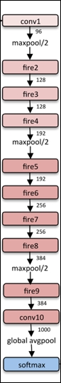
Figure 3: SqueezeNet architecture
You can download the Keras implementation of SqueezeNet (the squeezenet.py file) from the following link: https://github.com/rcmalli/keras-squeezenet.
Then we test the model on the following squeeze_test.jpg (227×227) image:

Figure 4: SqueezeNet test image
We do this by just using the following few lines of code:
import os
import numpy as np
import squeezenet as sq
from keras.applications.imagenet_utils import preprocess_input
from keras.applications.imagenet_utils import preprocess_input, decode_predictions
from keras.preprocessing import image


model = sq.SqueezeNet()
img = image.load_img('squeeze_test.jpg', target_size=(227, 227))
x = image.img_to_array(img)
x = np.expand_dims(x, axis=0)
x = preprocess_input(x)

preds = model.predict(x)
print('Predicted:', decode_predictions(preds))
As you can see, the results are very interesting:
Predicted: [[('n02504013', 'Indian_elephant', 0.64139527), ('n02504458', 'African_elephant', 0.22846894), ('n01871265', 'tusker', 0.12922771), ('n02397096', 'warthog', 0.00037213496), ('n02408429', 'water_buffalo', 0.00032306617)]]